LC-MS/MS Single Drug Quantification Guide

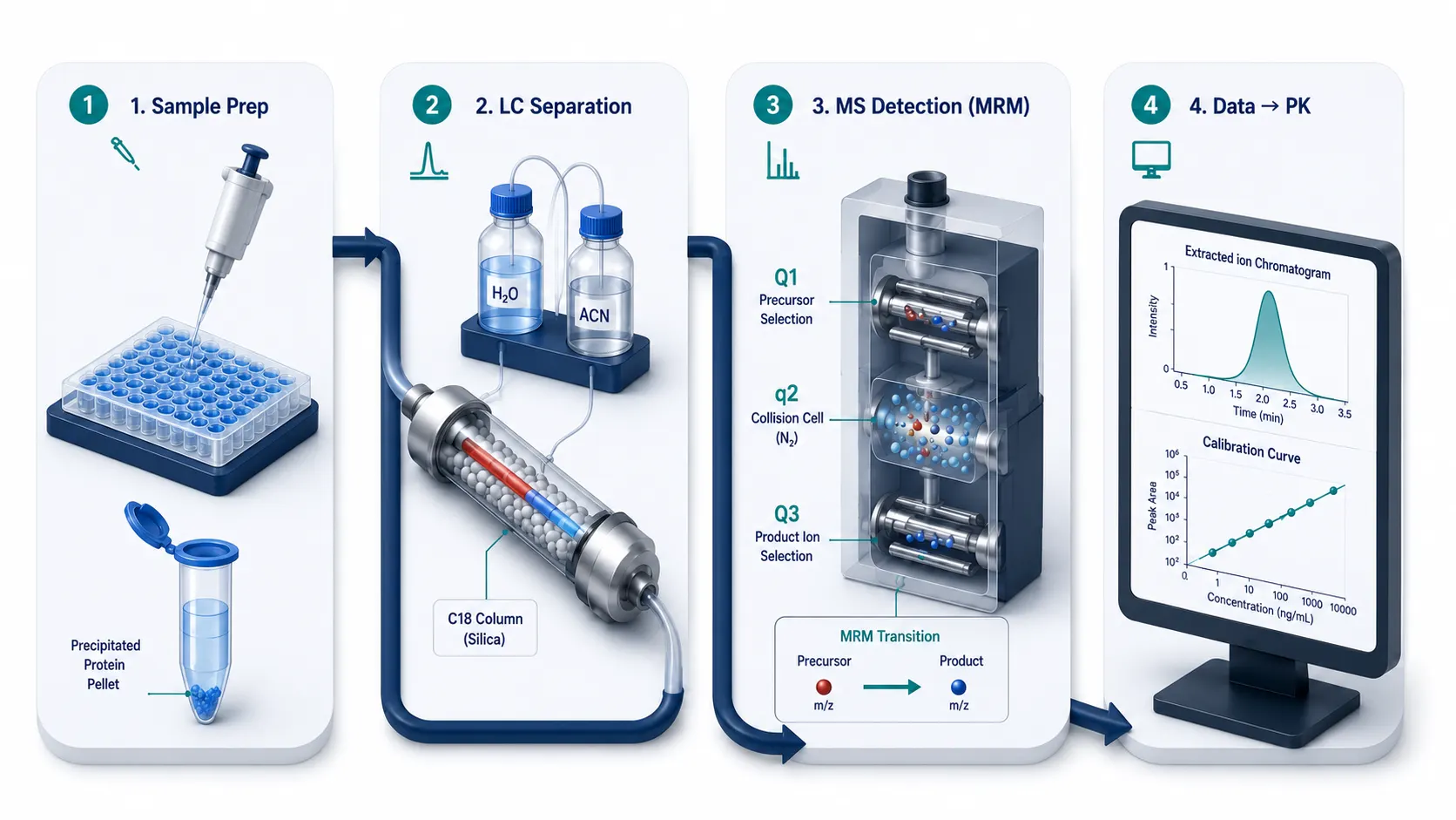
Figure 1: End-to-End LC-MS/MS Quantification Workflow — 3D Isometric Diagram

Why LC-MS/MS Remains the Gold Standard for Single Drug Quantification

In preclinical drug development, every pharmacokinetic conclusion depends on one number: the drug concentration in a biological sample. Get that number wrong, and you misjudge clearance, misread half-life, and misallocate millions in development capital. At Creative Proteomics, our DMPK bioanalysis platform provides ISO/IEC 17025-accredited LC-MS/MS single drug quantification services supporting drug discovery programs from lead optimization through IND-enabling studies. Liquid chromatography–tandem mass spectrometry (LC-MS/MS), operated on a triple quadrupole mass spectrometer in multiple reaction monitoring (MRM) mode, has been the undisputed gold standard for small-molecule quantification for over two decades — and for good reason.

Triple quadrupole MRM delivers three capabilities that no competing technology matches simultaneously. First, selectivity: by monitoring a precursor-to-product ion transition specific to the analyte, MRM discriminates the drug from thousands of co-extracted endogenous compounds with signal-to-noise ratios that UV-based detectors cannot approach. Second, sensitivity: modern triple quadrupole instruments routinely achieve lower limits of quantification (LLOQ) in the sub-ng/mL range from 50–100 µL of plasma — sufficient to characterize terminal elimination phases out to five half-lives. Third, dynamic range: calibration curves spanning four orders of magnitude (0.1–1000 ng/mL) with better than ±15% accuracy at all levels are standard for well-developed methods.

Compared to HPLC-UV, which lacks the selectivity to distinguish co-eluting metabolites from parent drug, LC-MS/MS eliminates the ambiguity. Compared to ELISA and other ligand-binding assays, which require validated antibody reagents that may cross-react with metabolites, LC-MS/MS provides unambiguous molecular specificity. Compared to GC-MS, which demands volatile, thermally stable analytes — or derivatization to make them so — LC-MS/MS handles polar, charged, and thermally labile compounds directly. The trade-off is capital cost: a triple quadrupole LC-MS/MS system represents a $300K–$600K investment, with annual maintenance and consumable costs of $100K–$200K. For most discovery programs, this cost is amortized across dozens of compounds and hundreds of studies, making per-sample costs competitive with — and often lower than — outsourced alternatives once throughput exceeds approximately 300–500 samples per month.

Preclinical bioanalysis imposes demands that clinical bioanalysis does not. Sample volumes are often limited to 25–50 µL of mouse or rat plasma, requiring the method to achieve target sensitivity from half the volume a clinical method would use. Throughput expectations are higher: a discovery PK study might generate 96 or 384 samples in a single dosing cohort, all needing results within 24–48 hours to inform the next round of medicinal chemistry. And the diversity of matrices — plasma, serum, whole blood, urine, bile, cerebrospinal fluid, and tissue homogenates from a dozen organ types — means the sample preparation and chromatography must be robust against matrix-to-matrix variability. Our complex biological matrices analysis services provide validated LC-MS/MS methods for tissue, CSF, bile, and cell lysate matrices that match the performance of our plasma-based methods. LC-MS/MS, alone among quantitative bioanalytical platforms, operates across all of these matrices with method adjustments rather than platform changes.

The Core LC-MS/MS Quantification Workflow: Four Stages

Every LC-MS/MS bioanalytical method, regardless of analyte, matrix, or regulatory context, follows the same four-stage architecture. Understanding what happens at each stage — and, more importantly, how decisions at one stage constrain options at the next — is the foundation of competent method development.

Stage 1 — Sample Preparation

The goal is deceptively simple: remove everything that is not the analyte while retaining all of the analyte. In practice, this means removing proteins (which would precipitate in the LC system and clog the column), phospholipids (the dominant source of ion suppression in electrospray ionization), salts, and other endogenous matrix components. The three primary approaches — protein precipitation (PPT), liquid-liquid extraction (LLE), and solid-phase extraction (SPE) — occupy different positions on the speed-versus-cleanliness spectrum. Selecting among them is the single highest-impact method development decision, and our sample preparation method development services systematically evaluate PPT, LLE, SPE, and SLE workflows to identify the optimal protocol for each analyte-matrix combination. This decision is explored in detail in Section 3.

Stage 2 — Chromatographic Separation

The liquid chromatography step separates the analyte from co-extracted matrix components in the time domain. Even with MRM selectivity, co-eluting matrix components — particularly phospholipids and salts — compete with the analyte for charge at the electrospray droplet surface, causing ion suppression that degrades both sensitivity and reproducibility. Chromatographic resolution between the analyte and these suppression-causing components is the most effective mitigation strategy, typically more robust than downstream MS parameter adjustments alone. Reversed-phase chromatography on C18 stationary phases, with acidic mobile phases (0.1% formic acid) and acetonitrile or methanol organic modifiers, is the default starting point for the vast majority of small-molecule drugs.

Stage 3 — Mass Spectrometric Detection (MRM)

The triple quadrupole mass spectrometer, operating in MRM mode, provides the analytical specificity. Q1 selects the precursor ion (typically [M+H]+ in positive ion mode for basic drugs, [M-H]− in negative ion mode for acidic drugs). The precursor is fragmented by collision-induced dissociation (CID) with nitrogen or argon gas in q2 (the collision cell). Q3 selects a structure-specific product ion. This two-stage mass filtering — precursor in Q1, product in Q3 — eliminates nearly all chemical noise, producing chromatograms where the analyte peak rises from a flat baseline. The MRM transition (precursor m/z → product m/z), collision energy, and dwell time are the three MS parameters that most directly influence sensitivity and must be optimized for each analyte.

Stage 4 — Data Processing and Quantification

The raw chromatographic data — analyte peak area, internal standard peak area, and their ratio — is processed through a calibration curve to produce a concentration value. Calibration curves are fitted by weighted linear regression (1/x² weighting is the industry-standard default, accounting for the heteroscedasticity of bioanalytical data — variance increases with concentration). The resulting concentration in ng/mL is multiplied by the sample dilution factor (if any) and reported. From concentration-time data across multiple sampling time points — whether from plasma and serum drug quantification or tissue and cell lysate analysis — non-compartmental analysis (NCA) yields the pharmacokinetic parameters — Cmax, Tmax, AUC, half-life, clearance, and volume of distribution — that drive development decisions. Each of these parameters is only as reliable as the concentration data that produced them.

Sample Preparation Strategy: PPT, LLE, or SPE? A Decision Framework

No single sample preparation technique is optimal for every analyte-matrix combination. The choice among protein precipitation (PPT), liquid-liquid extraction (LLE), and solid-phase extraction (SPE) — and, increasingly, supported liquid extraction (SLE) — is a multi-factorial decision that balances recovery, cleanliness, speed, cost, and the analytical requirements imposed by the target LLOQ and matrix complexity. Designing a method without a systematic framework for this decision is the most common root cause of methods that fail validation.

Protein Precipitation: When Speed Trumps Cleanliness

Protein precipitation is the simplest and fastest sample preparation technique. Add 3–4 volumes of organic solvent (typically acetonitrile or methanol, optionally acidified with 0.1% formic acid) to the biological sample, vortex briefly, centrifuge at 14,000g for 10 minutes, and inject the supernatant. The organic solvent disrupts the hydration shell around proteins, exposing hydrophobic cores that aggregate and precipitate, carrying down approximately 95–98% of protein mass. The entire process, from raw sample to injection-ready extract, takes under 30 minutes for a 96-well plate.

The trade-off is cleanliness. PPT removes proteins but leaves behind phospholipids, salts, and polar endogenous compounds that co-elute with the analyte in the early-eluting region of a reversed-phase gradient. Ion suppression from residual phospholipids — particularly lysophosphatidylcholines and phosphatidylcholines, which produce a characteristic m/z 184 product ion in positive ESI and affect a broad retention time window — can exceed 50% for early-eluting analytes. PPT is best suited for: (a) early discovery PK screening where throughput is paramount and 2–3-fold LLOQ variation is acceptable; (b) analytes with high MS sensitivity (sub-ng/mL on-column) where suppression can be tolerated; (c) matrices with relatively low phospholipid content, such as urine or cerebrospinal fluid; and (d) methods using a stable isotope-labeled internal standard (SIL-IS), which co-elutes with the analyte and compensates for suppression that occurs at the same retention time.

Liquid-Liquid Extraction: Selectivity for Lipophilic Compounds

LLE exploits differential solubility: the analyte partitions between an aqueous biological sample and a water-immiscible organic solvent based on its octanol-water partition coefficient (logP or logD at the extraction pH). Common extraction solvents include methyl tert-butyl ether (MTBE), ethyl acetate, hexane, and dichloromethane, selected based on the analyte's polarity and the solvent's selectivity for the compound class. After mixing and phase separation (by centrifugation or freezing), the organic layer is collected, evaporated to dryness under nitrogen, and reconstituted in an LC-compatible solvent.

LLE offers substantially better cleanup than PPT: phospholipids partition poorly into most LLE solvents in their ionized (zwitterionic) state, and proteins are completely excluded from the organic phase. This translates to lower ion suppression and cleaner chromatographic baselines. The limitation is polarity: compounds with logD < 0 at the extraction pH partition inefficiently into organic solvents, yielding recoveries below 60%. Highly polar drugs — including many carboxylic acid metabolites, Phase II conjugates (glucuronides, sulfates), and quaternary amines — are poor candidates for LLE. LLE is the method of choice for lipophilic drugs (logD > 1.5) when a structural analog internal standard (rather than SIL-IS) is used, because the improved matrix effect control reduces the IS-to-analyte response divergence that can occur under heavy suppression.

Solid-Phase Extraction: Maximum Matrix Removal for Demanding Assays

SPE passes the biological sample through a sorbent bed packed in a cartridge or 96-well plate. The analyte is retained by interactions with the sorbent (reversed-phase, ion-exchange, or mixed-mode) while matrix components are washed away. After washing, the analyte is eluted in a small volume of strong organic solvent. SPE provides the highest level of matrix removal — phospholipid removal exceeding 95% is achievable with polymeric and mixed-mode sorbents — and simultaneously concentrates the analyte, improving sensitivity by reducing the effective dilution factor compared to PPT.

The penalty is method development time and per-sample cost. SPE method development involves selecting the sorbent chemistry, optimizing the loading/washing/elution solvent composition and volumes, and verifying consistent recovery across the expected analyte concentration range. Per-sample consumable costs ($2–5) are 5–10× higher than PPT. SPE is indicated when: (a) the target LLOQ is below 0.5 ng/mL and every ionization efficiency gain matters; (b) the matrix is inherently dirty (tissue homogenates, fecal extracts, bile); (c) the analyte is highly polar (logD < 0) and cannot be extracted by LLE — ion-exchange SPE can retain and clean up charged analytes that LLE cannot touch; or (d) the method must meet ICH M10 validation criteria for a regulated study where matrix effect failures are unacceptable.

The Decision Tree

The optimal sample preparation technique is selected by answering four questions, in order:

1. What is the target LLOQ? If > 5 ng/mL in plasma, PPT (with SIL-IS) is usually sufficient. If 0.5–5 ng/mL, LLE or SPE should be considered. If < 0.5 ng/mL, SPE with concentration is the default starting point.
2. What is the compound's logD at physiological pH? If logD > 1.5, LLE is a strong candidate. If logD < 0, SPE (and specifically ion-exchange SPE for charged analytes) or PPT with SIL-IS are the remaining viable options.
3. What is the matrix? "Clean" matrices (urine, CSF, dialysate) — PPT is adequate. Plasma/serum — PPT with SIL-IS or LLE depending on LLOQ. Tissue homogenate, bile, feces — SPE is strongly recommended.
4. What is the regulatory stage? Discovery PK — PPT, optimize for speed. IND-enabling GLP tox — SPE or LLE, optimize for robustness. Regulated bioequivalence — method must pass full ICH M10 validation; invest in SPE method development upfront.

SLE and Automated 96-Well Workflows: The 2026 Efficiency Play

Supported liquid extraction (SLE) occupies a middle ground between LLE and SPE. The aqueous sample is loaded onto a diatomaceous earth sorbent bed where it spreads as a thin film. Organic solvent is passed through the bed, extracting the analyte from the aqueous film by LLE-like partitioning, but in a column format compatible with 96-well plates and liquid handlers. SLE avoids the emulsion formation that plagues traditional LLE, eliminates the phase separation step, and is readily automated. Combined with positive-pressure manifold processing, 96 samples can be prepared in under 60 minutes. For discovery and early preclinical programs processing more than 200 samples per week, automated SLE or 96-well SPE workflows deliver the best balance of matrix removal and throughput.

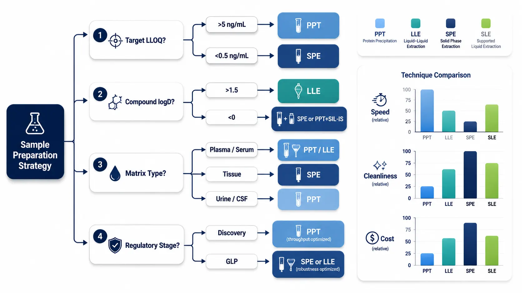Figure 2: Sample Preparation Decision Tree — PPT vs LLE vs SPE vs SLE

Chromatographic Optimization for Single Analyte Methods

Chromatography separates the analyte from matrix interferences in time. For single-analyte LC-MS/MS methods — where the entire gradient serves one compound — the optimization calculus is simpler than for multi-analyte panels, but the stakes are higher: every second of retention time costs throughput, and every co-eluting interference costs sensitivity.

Column Selection

C18 is the default stationary phase for > 80% of small-molecule drugs. For analytes with logD < 0 that elute near the void volume on C18, C8 (shorter alkyl chain, less retention) or embedded-polar-group C18 phases that tolerate 100% aqueous mobile phase can improve retention without switching to HILIC. Phenyl-hexyl phases provide pi-pi interactions with aromatic analytes, improving retention and selectivity for compounds with multiple aromatic rings. HILIC (hydrophilic interaction liquid chromatography) is reserved for very polar analytes (logD < −1) that show no retention on reversed-phase columns — but HILIC mobile phases (typically 70–95% acetonitrile) produce different ionization behavior in the ESI source, and method transfer between HILIC and reversed-phase is not straightforward.

Mobile Phase Optimization

For positive-ion ESI, the standard mobile phase is water (A) and acetonitrile or methanol (B), each containing 0.1% formic acid. Formic acid (pH ~2.7 in water) protonates basic analytes to form [M+H]+ and suppresses the ionization of acidic matrix components. For negative-ion ESI, 0.1% ammonium hydroxide or 5 mM ammonium acetate (pH ~6.8) deprotonates acidic analytes to form [M-H]−. The choice between acetonitrile and methanol affects both retention (acetonitrile is a stronger eluent — less is needed for equivalent retention) and ionization (methanol produces a different ESI droplet surface tension and evaporation rate, sometimes enhancing ionization for certain functional groups). Gradient slope controls the balance between separation and run time: a 2–4 minute gradient with a 0.3–0.5 mL/min flow rate on a 50 × 2.1 mm, 1.7–3 µm column achieves baseline separation for most single-analyte methods.

The 3-Minute Method: Speed vs. Resolution

Discovery PK demands turnaround times measured in hours, not days. The "3-minute method" — a 50 × 2.1 mm column, 0.5 mL/min flow rate, 5–95% organic gradient in 2 minutes, 1 minute re-equilibration — is the throughput standard. Achieving a 3-minute cycle while maintaining adequate resolution requires three conditions: (a) the analyte must elute at > 1.0 minutes (k' > 2) to avoid the suppression zone at the solvent front; (b) the internal standard must co-elute with the analyte (retention time difference < 0.1 min) for SIL-IS, or be baseline-resolved (> 0.3 min) for structural analogs; and (c) the carryover — measured by injecting a blank after the highest calibrator — must be < 20% of the LLOQ response. If any condition fails, extend the gradient to 4–5 minutes rather than accepting a defective method.

UPLC vs. HPLC: When Sub-2 µm Matters

UPLC (sub-2 µm particles, operating pressures of 8,000–15,000 psi) provides narrower peaks (peak width at half-height of 1–3 seconds vs. 5–10 seconds on HPLC), translating to higher signal-to-noise and better separation of the analyte from adjacent interference peaks. For methods targeting LLOQ < 0.5 ng/mL, UPLC provides 2–5× sensitivity improvement over HPLC on a 3–5 µm column, simply from peak concentration. For methods with adequate sensitivity on HPLC (LLOQ > 1 ng/mL), the throughput gain from UPLC is marginal — the gradient time, not the peak width, dominates the total run time — and the higher operating pressure increases column and instrument maintenance costs.

Internal Standard Strategy: SIL-IS vs. Structural Analogs

The internal standard is the single most important factor determining method precision. It corrects for: (a) variable recovery during sample preparation, (b) variable injection volume, (c) ionization efficiency drift within a batch, and (d) matrix effects that affect analyte and IS to the same degree (when the IS is properly chosen). A poorly chosen IS — or worse, no IS — converts these sources of variability directly into concentration errors. Choosing the right IS is not a formality; it is the difference between a method with ±3% precision and one with ±20% precision that fails validation.

SIL-IS: The Gold Standard

A stable isotope-labeled internal standard is the analyte molecule in which several hydrogen atoms (²H, deuterium), carbon atoms (¹³C), or nitrogen atoms (¹⁵N) are replaced by their stable heavy isotopes. The SIL-IS is chemically identical to the analyte — same functional groups, same ionization efficiency, same extraction recovery, same chromatographic retention time (or eluting within 0.03 minutes, the slight shift caused by deuterium's smaller van der Waals radius relative to hydrogen). Because the SIL-IS co-elutes with the analyte, it experiences exactly the same matrix environment at the moment of ionization. Any suppression or enhancement that affects the analyte affects the SIL-IS identically. The analyte-to-IS peak area ratio therefore remains constant regardless of matrix composition, injection precision, or MS sensitivity drift, producing the tightest possible precision (CV < 5% at mid-QC levels in a well-developed method).

SIL-IS has two limitations: cost and availability. A custom-synthesized ¹³C₆- or ²H₅-labeled analog typically costs $5,000–$25,000 for the initial synthesis, with lead times of 4–12 weeks. When SIL-IS is unavailable, our custom LC-MS/MS method development for novel chemical entities includes structural analog IS screening and validation to identify the optimal surrogate IS for your compound. For discovery programs testing dozens of structurally diverse compounds, synthesizing a SIL-IS for each is financially prohibitive. Deuterated analogs also exhibit a subtle chromatographic shift (deuterium isotope effect — ²H-labeled compounds elute 0.02–0.05 minutes earlier than the unlabeled analyte on C18 columns), which, while small, can cause differential matrix effects if a sharp suppression gradient exists at that retention time. ¹³C-labeled IS avoids this shift entirely (¹³C has the same van der Waals radius as ¹²C) and is preferred when available.

Structural Analog IS: When It Is the Right Call

A structural analog IS is a compound chemically similar to the analyte — a close homolog, a methylated/demethylated derivative, or a compound from the same chemical series — but not identical. It is available off-the-shelf at negligible cost relative to a custom synthesis. The structural analog IS should match the analyte in: (a) functional groups that determine ionization efficiency (same ionizable moiety), (b) logD (within 1–2 units), (c) retention time (eluting within 0.5–1.0 minutes, close enough to track similar matrix effects but resolved enough to avoid cross-talk).

Structural analog IS is appropriate when: (a) the method is for early discovery PK screening where ±15–20% accuracy is acceptable; (b) SIL-IS is not available and the cost/synthesis time is prohibitive; or (c) the structural analog has been validated to track the analyte's recovery and matrix effects within ±15% across multiple matrix lots. The validation experiment: spike analyte and analog IS at matched concentrations into ≥6 individual matrix lots, process independently, and compare the absolute IS response CV to the analyte response CV. If the IS response varies by more than 15% across lots, or if the analyte/IS peak area ratio CV exceeds the analyte response CV, the analog IS is not adequately tracking matrix effects, and SIL-IS or a different analog is required.

IS Addition Timing

The IS should be added as early as possible in the sample preparation workflow — ideally before or immediately after the first sample handling step. Adding IS before protein precipitation, LLE, or SPE allows it to correct for analyte loss throughout the entire process. Adding IS after extraction ("post-spike") corrects for MS variability and injection precision but not for extraction recovery — if recovery varies from sample to sample, that variation appears as concentration error. For regulated methods, IS is added to every sample, calibrator, and QC at the same concentration and at the same stage of processing.

Common IS Failure Modes

• Cross-talk: the IS MRM channel detects signal from the analyte (or vice versa) due to isotopic overlap or fragmentation in the ion source. Most common with single-²H-labeled IS where the M+1 isotopic peak of the analyte overlaps with the IS MRM channel. Fixed by using ¹³C₃₋₆ or ²H₃₋₅ labeled IS, or increasing chromatographic resolution between analyte and IS if using structural analog.
• IS degradation: the SIL-IS undergoes the same chemical degradation as the analyte during sample processing or storage. If degradation produces the unlabeled analyte as a degradation product, the measured concentration is inflated (especially near the LLOQ). Detect by incubating IS alone in matrix and measuring for analyte formation.
• Concentration mismatch: IS concentration is too low (peak area near noise, degrading precision at the high end of the calibration range) or too high (detector saturation, flat-topped peaks). IS concentration should produce a peak area approximately 40–60% of the ULOQ calibrator analyte peak area.
• Batch-to-batch IS variation: different lots of SIL-IS may have different isotopic purity (e.g., 98% vs. 99.5% ¹³C enrichment), changing the effective concentration. Qualify each new IS lot against the previous lot before use in a regulated study.

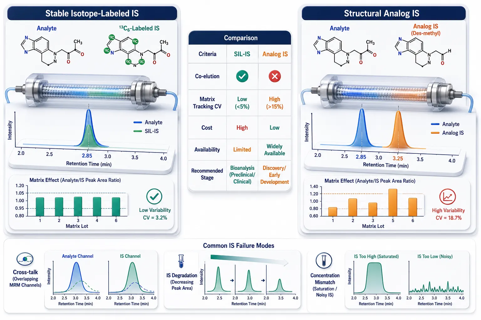Figure 3: SIL-IS vs Structural Analog Internal Standard — Co-Elution and Matrix Tracking Comparison

Pushing the LLOQ Lower: A Step-by-Step Guide

The lower limit of quantification (LLOQ) is the lowest concentration at which the analyte can be quantified with acceptable accuracy (±20%) and precision (CV ≤ 20%). For preclinical PK, the LLOQ determines how much of the terminal elimination phase the method can characterize — and thus how reliable the half-life and AUC extrapolation will be. A method with LLOQ = 5 ng/mL that loses the terminal phase after 24 hours produces a half-life estimate that is, at best, a lower bound. Pushing the LLOQ from 5 ng/mL to 0.5 ng/mL frequently doubles the number of quantifiable time points in the terminal phase and transforms the quality of the PK parameter estimates.

Start with the MS: MRM Optimization

Sensitivity optimization begins at the mass spectrometer. For each analyte, select the most abundant precursor ion (typically [M+H]+ in positive mode, [M-H]− in negative mode). Fragment the precursor at a range of collision energies (typically 10–50 eV in 5 eV steps) and select the product ion that provides the highest intensity. If two product ions have similar intensity, select the one with higher m/z (generally produces lower chemical noise). Optimize the declustering potential (or cone voltage, instrument-dependent), collision cell exit potential, and dwell time. Dwell time should be ≥ 30 ms for adequate sampling of the chromatographic peak (> 10 data points across the peak width); increasing dwell time beyond 100 ms provides diminishing returns unless the peak is very narrow (UPLC, < 3 seconds wide).

Upgrade Sample Preparation

If the MRM optimization is complete and the S/N at the desired LLOQ is still insufficient, the next step is improving the sample preparation. Switching from PPT to SPE (Section 3.3) does two things simultaneously: it reduces matrix suppression (increasing the absolute analyte signal at the LLOQ) and concentrates the sample (a typical SPE protocol concentrates the analyte 2–5× relative to PPT at the same sample volume). If SPE is already in use, increasing the sample volume and loading it onto the SPE cartridge — then eluting in the same final volume — is a linear sensitivity gain. Processing 200 µL of plasma and eluting in 50 µL (4× concentration) instead of 50 µL in 50 µL (1×) directly improves the LLOQ by a factor of 4.

Derivatization for Ionization Enhancement

For analytes with inherently poor ionization efficiency — low-proton-affinity compounds in positive mode, weakly acidic compounds in negative mode — chemical derivatization can improve sensitivity by 10–1,000×. Dansyl chloride derivatization of phenols and amines introduces a tertiary amine with high proton affinity, dramatically improving positive-ion ESI response. Picolinic acid or N-methylpyridinium derivatization of alcohols and carboxylic acids similarly boosts ionization. The cost is an additional sample preparation step (60–120 minutes of incubation, plus potential cleanup of excess reagent) and the complexity of a derivatization efficiency that must be consistent across calibrators, QCs, and study samples.

Microflow LC for Ultimate Sensitivity

Electrospray ionization is a concentration-sensitive technique: the signal depends on the analyte concentration in the sprayed solution, not the total mass of analyte. Reducing the chromatographic flow rate from 500 µL/min (analytical scale, 2.1 mm ID column) to 50–100 µL/min (microflow, 1.0 mm ID column) or 1–10 µL/min (nanoflow) concentrates the analyte into a smaller spray volume, increasing ionization efficiency. A 1.0 mm ID column at 100 µL/min typically provides 2–3× sensitivity improvement over a 2.1 mm column at 500 µL/min, with the same on-column mass. The trade-off: microflow systems are more susceptible to clogging, require cleaner extracts, have higher backpressure, and are less robust for high-throughput operation. Microflow is justified when the target LLOQ is < 0.1 ng/mL and all other optimization steps have been exhausted.

S/N ≥ 10 as the Real Target

ICH M10 specifies that the LLOQ signal-to-noise ratio should be ≥ 5. In practice, a method with S/N = 5 at the LLOQ will fail precision acceptance criteria at the LLOQ level (CV ≤ 20%) within 2–3 analytical runs because S/N drifts over time. A well-developed method targets S/N ≥ 10 at the nominal LLOQ during method development, providing adequate headroom for day-to-day instrument variability, column aging, and matrix lot-to-lot variation. Our full and partial method validation services include LLOQ verification across six individual matrix lots to confirm robustness before study sample analysis. If S/N = 10 cannot be achieved after exhausting the optimization steps above, raise the nominal LLOQ — an honest LLOQ of 2 ng/mL with S/N = 15 is far more defensible than a claimed LLOQ of 0.5 ng/mL with S/N = 4.

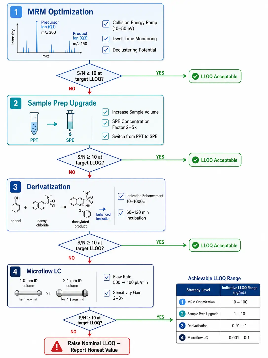Figure 4: LLOQ Optimization Flowchart — 4 Decision Nodes

Matrix Effects: From Mechanism to Mitigation

Matrix effects — the suppression or enhancement of analyte ionization by co-eluting matrix components — are the most common cause of bioanalytical method failure. Understanding the physicochemical mechanism is prerequisite to effective mitigation.

The Physics of Ion Suppression

In electrospray ionization, the analyte must reach the surface of the evaporating charged droplet, escape into the gas phase, and acquire a charge (the ion evaporation model for small molecules). Co-eluting nonvolatile matrix components — phospholipids, salts, proteins, and metabolites — compete for access to the droplet surface. Nonvolatile components accumulate on the droplet surface as the solvent evaporates, physically blocking analyte molecules from reaching the gas phase. Phospholipids are particularly effective suppressants because their amphiphilic structure (charged head group, hydrophobic tail) positions them ideally at the droplet surface. Salts suppress by increasing droplet surface tension and conductivity, changing the droplet fission dynamics. The net effect: fewer analyte ions reach the detector per unit time, reducing the observed signal — the peak area — by 10–90% depending on the matrix component identity, concentration, and chromatographic overlap with the analyte.

APCI vs. ESI Sensitivity to Matrix Effects

Atmospheric pressure chemical ionization (APCI) is substantially less susceptible to matrix effects than ESI because the ionization mechanism is different. In APCI, the analyte is vaporized by heating, then ionized in the gas phase by charge transfer from solvent reagent ions — there is no charged droplet, no competition for the droplet surface. However, APCI requires the analyte to be thermally stable and volatile, which excludes many drug classes (glucuronide conjugates, quaternary amines, high-molecular-weight compounds). APCI is worth evaluating when: (a) the analyte is amenable (MW < 800, thermally stable, some volatility); (b) matrix effects exceed 30% suppression despite optimized chromatography and sample preparation; and (c) the required LLOQ is > 1 ng/mL (APCI is typically 2–5× less sensitive than ESI for the same analyte).

The Mitigation Pyramid

Matrix effect mitigation is hierarchical, with each level addressing the problem at a different point in the analytical workflow:

1. Chromatography (most effective): separate the analyte from the suppression-causing matrix components. Phospholipids elute in a characteristic retention window (typically 60–90% organic on a C18 gradient). If the analyte is retained beyond this window — through column selection, gradient adjustment, or mobile phase modification — it never encounters the suppressant at the ESI source. This is the most robust strategy because it physically separates the problem rather than compensating for it.
2. Sample preparation: remove suppressants before they reach the LC system. SPE with polymeric or mixed-mode sorbents removes > 95% of phospholipids. LLE excludes phospholipids from the organic extract.
3. Internal standard compensation: a co-eluting SIL-IS experiences the same suppression as the analyte, so the peak area ratio is preserved. This is compensation, not mitigation — the absolute signal is still suppressed — but the quantification is unaffected. Structural analog IS that elutes at a different retention time may experience different suppression and fail to compensate.
4. Source switching: evaluate APCI if ESI suppression is intractable.
5. Online SPE / turbulent flow chromatography: automated sample cleanup directly coupled to the LC-MS/MS system, removing matrix components online without manual sample preparation. High capital cost but maximum robustness for very high-throughput regulated methods.

Assessing Matrix Effects per ICH M10

ICH M10 requires matrix effect assessment using ≥ 6 individual matrix lots (from different individuals). For each lot, the matrix factor (MF) is calculated as: MF = peak area of analyte in post-extraction spiked matrix / peak area of analyte in neat solution. The IS-normalized MF = MF_analyte / MF_IS. The CV of the IS-normalized MF across all lots should be ≤ 15%. If one or two lots exceed this threshold, the method may still be acceptable if the majority of lots pass. When persistent matrix effect failures occur — particularly with complex matrices — our endogenous interference resolution services apply advanced chromatography and selective sample preparation to eliminate co-eluting suppressants. For a deeper treatment of matrix effect mechanisms — including post-column infusion assessment, phospholipid profiling, and lot-to-lot variability strategies — see our dedicated guide on bioanalytical matrix effect evaluation and mitigation. The ICH M10 validation framework, including full validation parameter checklists and acceptance criteria tables, is covered in a separate resource on regulatory bioanalytical method validation.

Understanding ICH M10 Method Validation: What It Means for Preclinical Data Quality

ICH M10, adopted in 2022, is the harmonized global standard for bioanalytical method validation. It consolidates and replaces previous regional guidance (FDA 2018 BMV Guidance, EMA 2011 BMV Guideline, Japan MHLW 2013 BMV Guideline) into a single framework. For preclinical scientists, ICH M10 is simultaneously the quality benchmark to aspire to and a regulatory reality to navigate pragmatically depending on development stage.

ICH M10 as Industry Knowledge

ICH M10 specifies the validation parameters that must be assessed — selectivity, specificity, calibration model, accuracy and precision, matrix effect, dilution integrity, carryover, and stability — and the acceptance criteria for each. The standard accuracy and precision criterion is ±15% (±20% at LLOQ). Calibration curves must contain ≥ 6 non-zero calibrators and meet back-calculated accuracy within ±15% (±20% at LLOQ), with ≥ 75% of calibrators meeting criteria. Stability must be assessed under all conditions to which study samples will be exposed: bench-top stability (matrix), freeze-thaw stability (≥ 3 cycles), long-term frozen storage stability, stock and working solution stability, autosampler stability (processed sample), and whole blood stability (when there is a delay between collection and centrifugation).

Understanding ICH M10 is essential for anyone conducting bioanalysis — whether or not the specific study requires full compliance — because the principles it codifies (matrix effect assessment, stability characterization, calibration model quality) represent good bioanalytical practice regardless of regulatory context. A method that would fail ICH M10 is a method that produces unreliable data, GLP or not.

Core Validation Parameters

• Accuracy and Precision: within-run and between-run, assessed at four QC levels (LLOQ, Low QC, Mid QC, High QC), ≥ 3 analytical runs, ≥ 5 replicates per QC per run.
• Selectivity: ≥ 6 individual matrix lots, blank matrix should show no significant interference (< 20% of LLOQ response and < 5% of IS response) at the analyte retention time.
• Calibration Model: the relationship between concentration and response should be continuous and reproducible. Weighted (1/x²) linear regression is standard. The model must be validated across the intended concentration range.
• Carryover: response in a blank sample injected after the highest calibrator (ULOQ) must be < 20% of the LLOQ response for the analyte and < 5% for the IS.
• Dilution Integrity: if study samples will be diluted, the dilution procedure must be validated by diluting QC samples above the ULOQ with blank matrix to bring them within the calibration range. Accuracy and precision at the diluted concentration must meet ±15%.

GLP vs. Non-GLP Bioanalysis: Matching Rigor to Development Stage

Not every bioanalytical study needs GLP compliance. GLP (Good Laboratory Practice, 21 CFR Part 58) is a regulatory quality system governing the organizational process and conditions under which non-clinical laboratory studies are planned, performed, monitored, recorded, and reported. GLP compliance is mandatory for safety studies that support IND/NDA submissions — specifically, pivotal toxicology studies where bioanalytical data will be used to establish exposure-toxicity relationships that inform clinical starting doses and safety margins.

For discovery PK screening, lead optimization, early ADME characterization, and mechanism-of-action studies, GLP compliance is regulatory overkill. Our bioanalytical method development and validation services provide fit-for-purpose validation under ISO/IEC 17025 accreditation — delivering regulatory-grade data quality with the speed and flexibility discovery programs require. It adds 2–4 weeks to study timelines (SOP documentation, quality assurance unit review, formal study protocol and report), increases costs by 30–50%, and reduces the flexibility to adapt methods as new data emerges — all for studies whose data will never appear in a regulatory submission module. The key decision criterion: will this specific bioanalytical dataset be submitted to a regulatory agency to support a safety or efficacy claim? If yes, GLP (or GCP for clinical) applies. If no, fit-for-purpose validation in an ISO 17025-accredited laboratory provides the appropriate balance of data quality, speed, and cost.

ISO 17025 Accreditation: What It Certifies

ISO/IEC 17025 is the international standard for testing and calibration laboratory competence. Accreditation certifies that the laboratory: (a) operates a quality management system with documented SOPs, controlled documents, and corrective/preventive action procedures; (b) employs technically competent staff with documented training and qualification records; (c) uses calibrated and maintained instruments with documented calibration traceability; (d) participates in proficiency testing programs; and (e) validates analytical methods before placing them into service. Critically, ISO 17025 certifies the laboratory's technical competence — it is not a substitute for GLP or GCP in regulatory submissions, but it provides an independently audited assurance that the concentration data produced by the laboratory is technically sound.

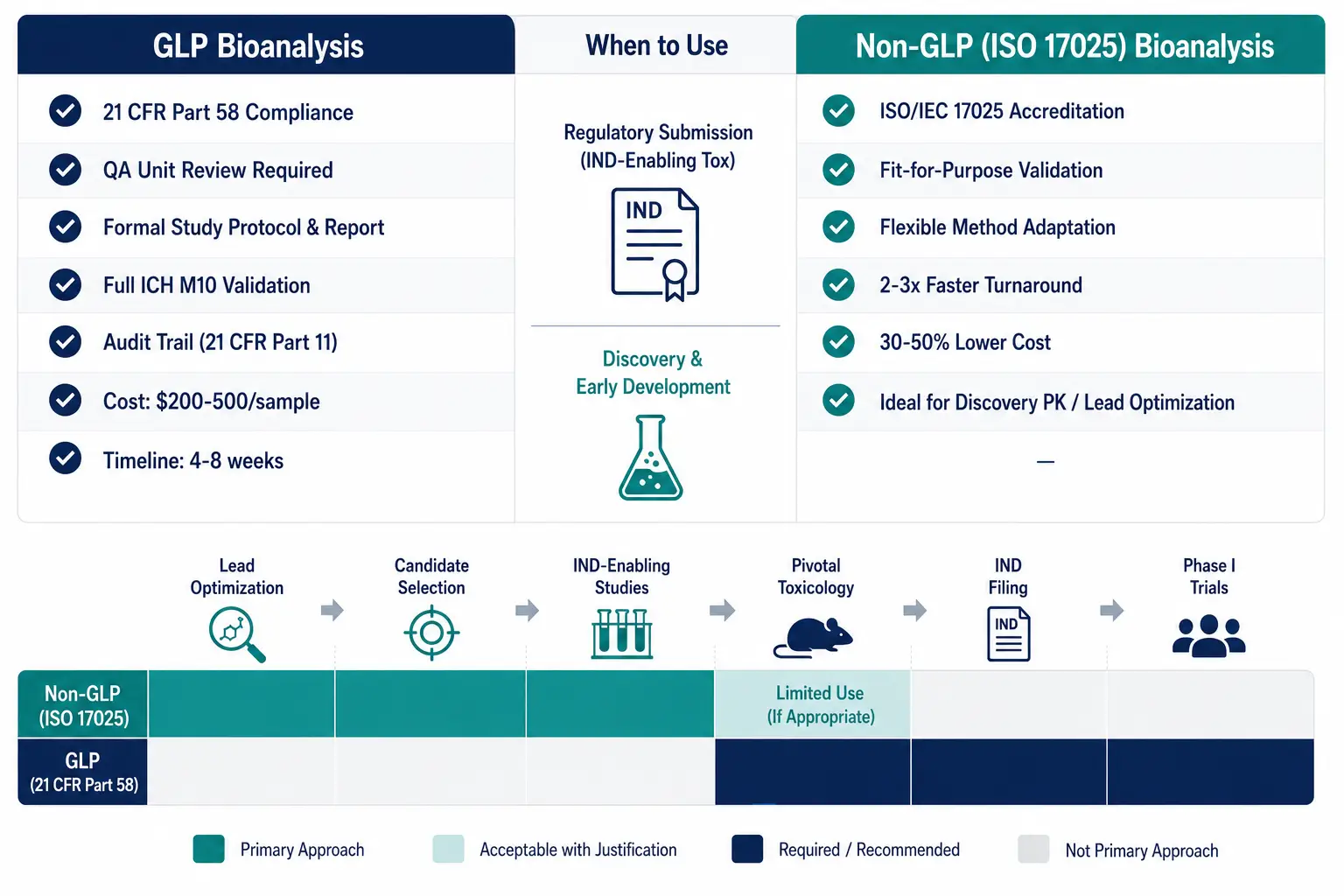Figure 5: GLP vs Non-GLP Bioanalysis — Comparison Matrix

From Bench to Report: Data Processing and PK Parameters

The chromatographic peak integration and calibration curve that produce a concentration value are the bridge between the analytical chemistry and the pharmacokinetic interpretation. Errors at this stage — incorrect integration, improper calibration curve weighting, manual integration without documentation — propagate directly into PK parameters and, ultimately, into development decisions.

Calibration Curve Fitting

Bioanalytical calibration curves are heteroscedastic: the absolute variance of the response increases with concentration. Ordinary least squares (unweighted) regression gives disproportionate influence to the high-concentration calibrators, producing systematic bias at the low end of the curve — the region that determines the LLOQ and the terminal-phase concentrations most critical for half-life estimation. Weighted linear regression with 1/x² weighting normalizes the heteroscedasticity, giving each calibrator level approximately equal influence on the fitted line. The calibration model is acceptable if ≥ 75% of calibrators back-calculate to within ±15% (±20% at LLOQ) of their nominal concentration.

Key PK Parameters and Their Bioanalytical Dependencies

• Cmax and Tmax: directly observed from the concentration-time data. Cmax is only as reliable as the sampling schedule — if the true Tmax falls between two sampling points, Cmax is underestimated. Adequate sampling density around the expected Tmax (typically 2–4 time points in the absorption phase) is essential.
• AUC (Area Under the Curve): calculated by the trapezoidal rule from the concentration-time data. AUC extrapolation from Tlast to infinity (AUC_extrap) should be ≤ 20% of the total AUC for the half-life estimate to be considered reliable. If LLOQ limitations mean the terminal phase is incompletely captured, AUC is underestimated and the extrapolation percentage is inflated — a bioanalytical problem masquerading as a PK one.
• t½ (Terminal Half-Life): calculated as 0.693/λz, where λz is the terminal elimination rate constant estimated from the slope of ln(concentration) vs. time. λz estimation requires ≥ 3 concentration values in the terminal phase (preferably ≥ 4), spanning at least one half-life, with r² ≥ 0.85 for the regression. The lowest quantifiable concentration must be well above the LLOQ.
• CL (Clearance) and Vd (Volume of Distribution): calculated from AUC and dose (CL = Dose/AUC; Vd = CL/λz). These parameters carry forward every error in the concentration data — a 20% negative bias in AUC produces a 25% positive bias in CL.

Non-Compartmental Analysis (NCA) Fundamentals

NCA is the standard method for PK parameter estimation from in vivo data. It makes no assumptions about the number of body compartments; it calculates parameters directly from the concentration-time data using the statistical moment theory. The two primary outputs are: (a) the area under the curve (AUC, zeroth moment), reflecting total drug exposure; and (b) the mean residence time (MRT, first moment / zeroth moment), reflecting the average time a drug molecule spends in the body. NCA is robust, regulatorily accepted, and implementable by any validated software (Phoenix WinNonlin, PK Solver, or R-based packages). A deeper treatment of NCA methodology — including λz selection rules, trapezoidal rule variants, and strategies for handling sparse sampling data — can be found with our guide to plasma drug concentration-time curve interpretation and PK parameter estimation.

Documentation and Data Integrity

Every manual integration, every excluded calibrator, every reinjected sample must be documented with a justification that would be intelligible to an auditor three years later. "Peak integration adjusted due to interference" is insufficient; "Interference peak at 2.45 min, identified as phospholipid m/z 184→184, resolved by manual integration from 2.40–2.50 min — see chromatogram in batch file XYZ" is acceptable. For regulated studies, the FDA's 21 CFR Part 11 and equivalent international regulations require secure, computer-generated, time-stamped audit trails that independently record the date, time, and operator of every data manipulation. The ICH M10 validation framework — including full parameter checklists, acceptance criteria, and documentation requirements for regulated bioanalysis — is detailed in a dedicated resource on regulatory method validation.

In-House vs. Outsourced LC-MS/MS Bioanalysis: Matching Strategy to Development Stage

The decision to build in-house LC-MS/MS capability or outsource to a CRO is not primarily technical — it is strategic. Both approaches produce valid concentration data. The deciding factors are capital, throughput, timeline, and the intangible cost of diverting internal expertise from the core scientific mission.

The Economics

Building an in-house bioanalytical laboratory requires: one or more triple quadrupole LC-MS/MS systems ($300K–$600K capital per system), a dedicated laboratory space with controlled temperature/humidity, solvent storage, and waste handling, at least one full-time experienced bioanalytical scientist ($80K–$150K annual salary plus benefits), and annual operating costs (consumables, maintenance contracts, proficiency testing) of $50K–$100K per instrument. The all-in annual cost for a single-instrument laboratory is approximately $200K–$350K. At a typical CRO per-sample cost of $50–$150 for discovery PK and $200–$500 for regulated bioanalysis, the break-even point is roughly 2,000–3,000 samples per year. Below this threshold, outsourcing is almost always more cost-effective. Above it, in-house capability begins to offer a return on investment.

When In-House Wins

In-house bioanalysis is advantageous when: (a) annual sample volume exceeds the break-even threshold and is expected to remain there; (b) turnaround time is critical — in-house samples can be processed and results returned in 24–48 hours, compared to 1–2 weeks typical for outsourced studies; (c) the compound series requires iterative method development tightly coupled to medicinal chemistry (method parameters change with each new analog, and the bioanalyst needs to understand the structure-activity relationships to optimize accordingly); and (d) the intellectual property sensitivity is high (novel chemical matter where compound structure disclosure to an external party is undesirable before patent filing).

When Outsourcing Wins

Outsourcing to a CRO is the better choice when: (a) annual sample volume is below the break-even threshold; (b) the organization is a virtual biotech without physical laboratory infrastructure; (c) the required expertise is specialized and infrequently needed (e.g., tissue drug quantification requiring specific homogenization and extraction expertise, or large-molecule LC-MS/MS); (d) capacity overflow — internal laboratory is at full capacity and additional instrument investment is not justified by the overflow volume; or (e) the study is a one-off regulatory submission where the CRO's established GLP compliance program and regulatory inspection history provide risk mitigation.

Choosing the Right Partner

The first question to ask a prospective CRO is: "What regulatory quality system is appropriate for this specific study?" The answer should distinguish between full GLP compliance (for IND-enabling tox studies), ISO 17025-accredited non-GLP work (for discovery and preclinical research), and fit-for-purpose exploratory work (for early screening). If the CRO defaults to GLP for everything, they may be inflating costs unnecessarily. If they cannot provide GLP when you need it, they cannot support your regulatory submissions. A specialized DMPK-focused CRO such as Creative Proteomics, operating under ISO/IEC 17025 accreditation with deep expertise in LC-MS/MS method development across plasma, serum, tissue, and cell lysate matrices, offers both tracks and helps sponsors select the appropriate quality system based on development stage and regulatory requirements.

Supporting services such as in vitro compound stability and forced degradation profiling and high-resolution metabolite quantification should be available from the same CRO to avoid the data fragmentation that occurs when different providers handle different portions of the bioanalytical workflow. Other evaluation criteria include: (a) demonstrated experience with your specific matrix type and analyte class (ask for anonymized case studies); (b) data integrity infrastructure — 21 CFR Part 11 compliant data systems with full audit trails; (c) method development timeline commitments (discovery methods in < 2 weeks, regulated methods in < 6 weeks); (d) communication protocols — how and when are analytical issues communicated?; and (e) regulatory inspection history — has the CRO been inspected by FDA/EMA, and what were the outcomes?

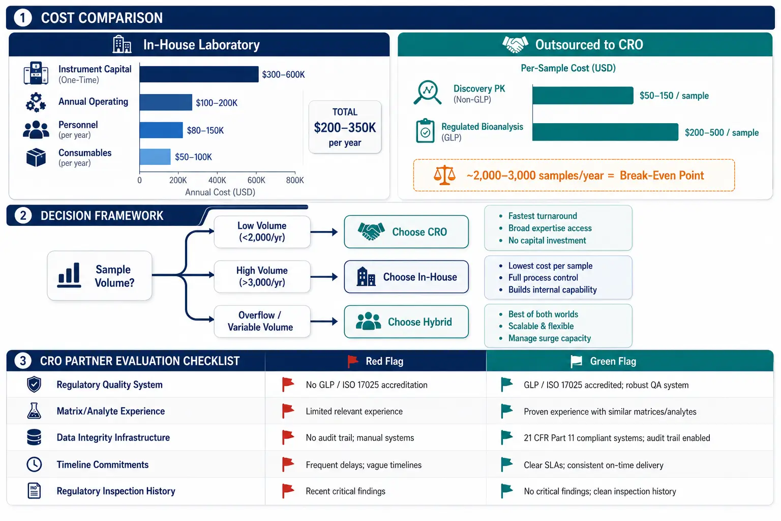Figure 6: In-House vs Outsourced Bioanalysis — Decision Framework

What Is Next: 2026 Technology Trends

LC-MS/MS bioanalysis is not static. Five technology trends are reshaping the field as of 2026, each with implications for preclinical drug quantification.

Microflow LC: Sensitivity Without Nanoflow Fragility

Microflow LC (0.3–1.0 mm ID columns, 10–100 µL/min flow rates) occupies the practical middle ground between analytical-scale LC (2.1 mm ID, 300–600 µL/min) and nanoflow LC (< 0.1 mm ID, < 1 µL/min). It provides 2–5× sensitivity improvement over analytical-scale LC through concentration of the analyte in a smaller spray volume, while maintaining the robustness required for high-throughput operation. Microflow systems with plug-and-play fluidics and integrated column ovens have matured to the point where they are viable for routine use, not just specialist applications. The 2026 commercial landscape includes microflow platforms from all major MS vendors, with factory-optimized source configurations that eliminate the manual tuning previously required.

HRMS Entering Routine Quantitation

High-resolution mass spectrometry (Q-TOF and Orbitrap) has historically been the domain of qualitative analysis — metabolite identification, proteomics, and untargeted screening. In 2026, the sensitivity gap between HRMS and triple quadrupole MRM has narrowed to within 2–5× for most analytes, and HRMS offers a compelling advantage: full-scan acquisition with post-hoc extraction of any ion chromatogram. For studies requiring simultaneous quantitation of parent drug and structural elucidation of metabolites, a single HRMS injection replaces two separate analyses (triple quadrupole for quantitation + Q-TOF for metabolite ID). For discovery programs, the ability to retrospectively mine HRMS data for metabolites, biomarkers, or unexpected adducts without re-running samples is a substantial efficiency gain.

AI-Assisted Data Processing

Automated peak integration has been available for decades, but AI/ML-based approaches are now moving beyond automation into intelligence: flagging integrations that are likely incorrect based on learned chromatographic patterns, detecting systematic batch drift before it exceeds acceptance criteria, and predicting method parameters (MRM transitions, collision energies, gradient conditions) from compound structure. These tools augment, rather than replace, the experienced bioanalyst — they reduce the time spent on routine data review and flag the cases that genuinely require human judgment. The 2026 state of the art is "human-in-the-loop" AI, where algorithm-processed data is presented with confidence scores, and only low-confidence integrations are referred for manual review.

Microsampling for Rodent PK

Dried blood spot (DBS) and volumetric absorptive microsampling (VAMS) collect 10–30 µL of blood from a tail-vein or saphenous-vein puncture, eliminating the need for terminal blood collection in rodents and enabling serial sampling from the same animal. This reduces animal use by 60–80% (serial sampling from n=3 vs. composite sampling from n=15) while producing individual — rather than composite — PK profiles. The bioanalytical challenge is sensitivity: the collected blood volume is 5–10× smaller than a conventional plasma sample, requiring the LC-MS/MS method to achieve the same LLOQ from proportionally less matrix. The combination of microflow LC with VAMS sampling is a natural pairing that is gaining adoption in discovery PK workflows. Our microsampling bioanalysis services support DBS and VAMS-based PK studies with validated LC-MS/MS methods optimized for the 10–30 µL sample volumes these techniques generate.

Hybrid LBA–LC-MS/MS

Ligand-binding assay (LBA) capture followed by LC-MS/MS detection combines the selectivity of immunoaffinity enrichment with the specificity of mass spectrometric quantification. The primary application is for large molecules (therapeutic proteins, monoclonal antibodies, ADCs) where ELISA alone cannot distinguish the intact drug from metabolites or anti-drug antibody complexes. For small molecules, LBA–LC-MS/MS is used when extreme sensitivity is required (femtogram/mL LLOQ) — the antibody enriches the analyte from a large sample volume, and the LC-MS/MS provides the specific readout. This is a niche technique for preclinical bioanalysis (applied primarily to biologics and ultrasensitive biomarker panels) but is growing in importance as the drug development pipeline shifts toward biologics and protein therapeutics.

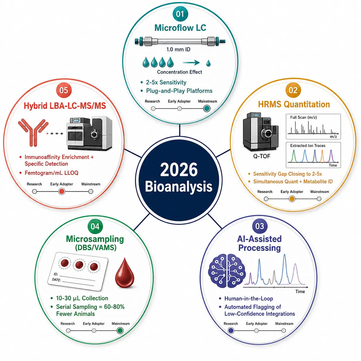Figure 7: 2026 Technology Landscape — Five Emerging Trends in LC-MS/MS Bioanalysis

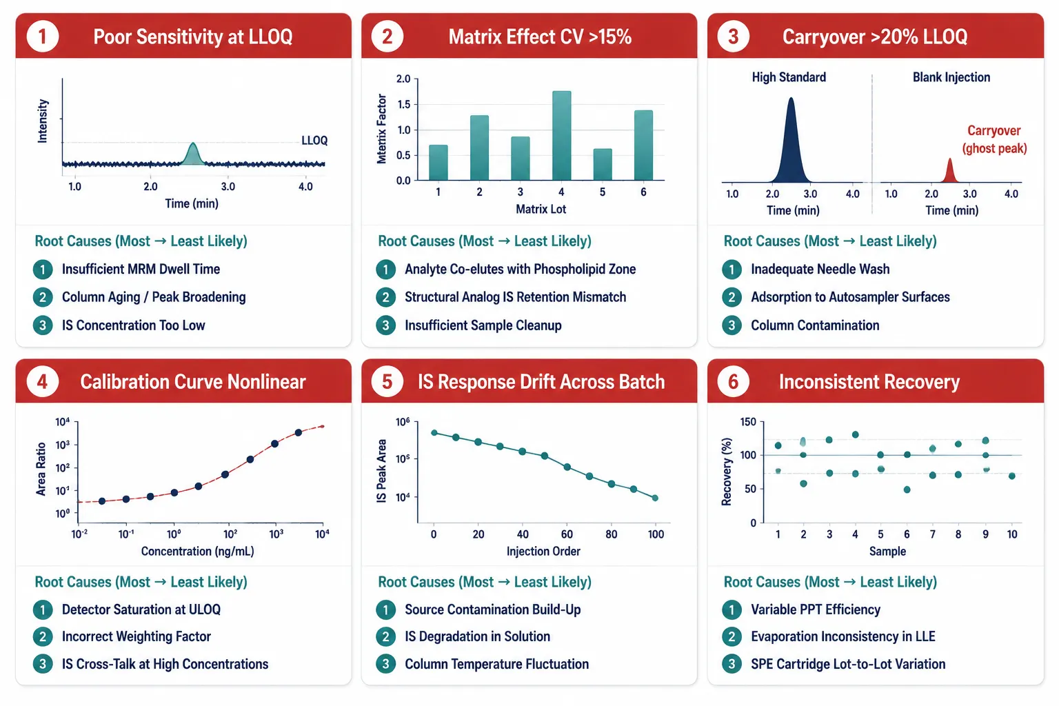Figure 8: Troubleshooting Reference — Common LC-MS/MS Method Failures and Root Causes

Frequently Asked Questions

References

Related Services

• Single Drug Quantification by LC-MS/MS
• Bioanalytical Method Development & Validation
• Custom Method Development for NCEs
• Sample Preparation Workflow Optimization
• Full & Partial Method Validation
• Plasma & Serum Drug Quantification
• Tissue & Cell Lysate Drug Quantification
• Complex Biological Matrices Analysis
• Compound Stability & Forced Degradation Profiling
• Microsampling Bioanalysis

References

- ICH Harmonised Guideline. Bioanalytical Method Validation and Study Sample Analysis M10. International Council for Harmonisation of Technical Requirements for Pharmaceuticals for Human Use; 2022.
- Matuszewski BK, Constanzer ML, Chavez-Eng CM. Strategies for the assessment of matrix effect in quantitative bioanalytical methods based on HPLC-MS/MS. Analytical Chemistry. 2003;75(13):3019-3030.
- Van Eeckhaut A, Lanckmans K, Sarre S, Smolders I, Michotte Y. Validation of bioanalytical LC-MS/MS assays: evaluation of matrix effects. Journal of Chromatography B. 2009;877(23):2198-2207.
- Jemal M, Ouyang Z, Xia YQ. Systematic LC-MS/MS bioanalytical method development that incorporates plasma phospholipids risk avoidance, usage of incurred sample and well thought-out chromatography. Biomedical Chromatography. 2010;24(1):2-19.
- Korfmacher WA. Foundation review: principles and applications of LC-MS in new drug discovery. Drug Discovery Today. 2005;10(20):1357-1367.
- Hendrikx JJMA, Dubbelman AC, Rosing H, Schinkel AH, Schellens JHM, Beijnen JH. Quantification of docetaxel and its metabolites in human plasma by liquid chromatography/tandem mass spectrometry. Rapid Communications in Mass Spectrometry. 2013;27(17):1925-1934.
- Xu RN, Fan L, Rieser MJ, El-Shourbagy TA. Recent advances in high-throughput quantitative bioanalysis by LC-MS/MS. Journal of Pharmaceutical and Biomedical Analysis. 2007;44(2):342-355.
- Bonfiglio R, King RC, Olah TV, Merkle K. The effects of sample preparation methods on the variability of the electrospray ionization response for model drug compounds. Rapid Communications in Mass Spectrometry. 1999;13(12):1175-1185.
- De Nicolò A, Cantù M, D'Avolio A. Matrix effect management in liquid chromatography mass spectrometry: the internal standard normalized matrix effect. Bioanalysis. 2017;9(14):1093-1105.
- Taylor PJ. Matrix effects: the Achilles heel of quantitative high-performance liquid chromatography-electrospray-tandem mass spectrometry. Clinical Biochemistry. 2005;38(4):328-334.