Every pharmacokinetic report contains at least one concentration-time curve. The curve is not decoration — it is the primary data visualization. Before any parameter is calculated, the curve carries the answer. A trained eye can estimate Cmax, judge absorption rate, and spot problems (flip-flop kinetics, enterohepatic recirculation, sampling gaps) from the curve alone. This article explains how to read plasma drug concentration-time curves the way experienced PK scientists do — by understanding shape, scale, and what each feature implies about the drug's behavior.
The Anatomy of a Concentration-Time Curve
A plasma concentration-time curve after oral dosing has three visually distinct regions, each governed by a different physiological process.
The Absorption Phase — The Rising Limb
From time zero to Cmax, the curve rises. The steepness of this rise reflects the absorption rate constant (ka). A steep, early peak (Tmax < 1 h) means gastric emptying and intestinal permeability are not rate-limiting — the drug crosses the gut wall quickly. A broad, late peak (Tmax 3-6 h) suggests slow or sustained absorption: poor solubility, controlled-release formulation, or transporter-mediated uptake that saturates.
A practical rule: if two sampling points bracket the true peak, Cmax is captured adequately. If the first sample is the highest, Cmax is unreliable — the peak occurred before the first blood draw. In preclinical PK, add a 15-minute time point for rats and a 5-10 minute point for mice to avoid this.
The Distribution Phase — The Bend
After Cmax, the curve declines rapidly for a period before settling into a straight-line slope on a semi-log plot. This initial rapid decline is the distribution phase: drug is simultaneously being eliminated and distributing from plasma into tissues. The curve bends because two processes (distribution + elimination) are occurring. Once distribution equilibrium is reached, only elimination governs the decline — and the curve becomes log-linear.
The bend is most prominent for drugs with moderate-to-large Vd. For drugs confined to plasma (Vd ≈ 3-5 L), the distribution phase is barely visible. For tissue-binding drugs (Vd > 100 L), the distribution phase can dominate the first several hours of the curve. Recognizing where distribution ends and elimination begins is essential because the terminal slope for half-life calculation must be taken from the elimination phase only — including distribution-phase points shortens the apparent half-life.
The Elimination Phase — The Straight Line on Semi-Log
On a semi-log plot (log concentration vs linear time), first-order elimination produces a straight line. The slope of this line is the elimination rate constant (kel or λz). Half-life = ln(2) / kel.
A log-linear curve requires at least 3 points — preferably 4-5 — in the terminal phase. Two points define a line but provide no diagnostic information about whether the slope is being distorted by a late-absorbing fraction or assay variability at low concentrations. Each additional terminal-phase point increases the reliability of the half-life estimate. For reliable AUC extrapolation, the last measurable concentration should be below 20% of Cmax and the extrapolated area should contribute less than 20% of total AUC.
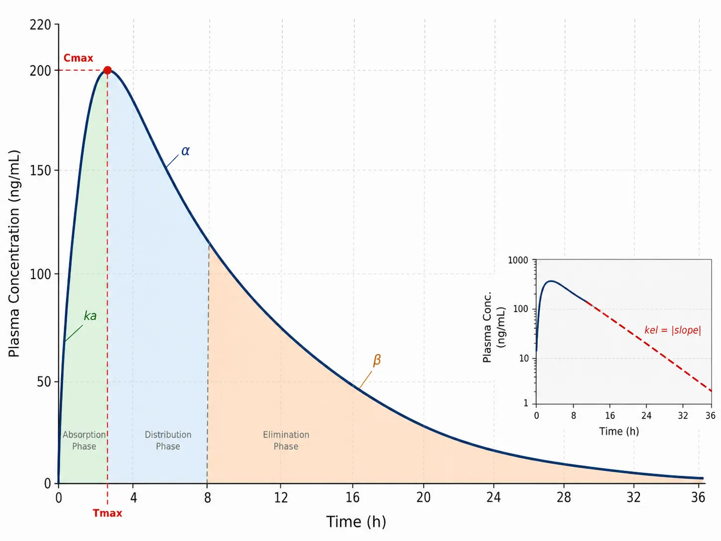 Figure 1: Three-phase anatomy of an oral concentration-time curve — absorption (rising limb, labeled ka), distribution (curved decline post-Cmax, labeled α phase), and elimination (straight-line terminal decline on semi-log inset, labeled β phase with kel). Main plot: linear scale showing all three phases. Inset: same data on semi-log scale showing the straight terminal line.
Linear vs Semi-Log: Why the Log Scale Matters
Pharmaceutical scientists present concentration-time data on two scales, and the choice determines what information is immediately visible.
Linear Scale
Used for IV bolus data and for assessing overall curve shape. On a linear plot, first-order elimination produces an exponential decay — the curve approaches zero asymptotically. AUC is directly visible as the area under the curve. Cmax and Tmax are read at a glance. The limitation: the terminal phase is compressed near zero, making it difficult to judge whether elimination is truly log-linear or to identify late-time anomalies.
Semi-Log Scale
The same data plotted as log(concentration) vs linear time. First-order elimination now appears as a straight line. This is the essential transformation for PK analysis because: (1) half-life is directly visible as the time required for concentration to halve along the straight segment; (2) deviations from log-linearity — saturation kinetics, auto-induction, multi-exponential elimination — are immediately apparent as curvature; (3) extrapolation to infinity for AUC calculation is performed on the log-linear fit.
Common practice: present curves on linear scale in reports but verify terminal log-linearity on semi-log. A curve that looks unremarkable on a linear plot may reveal a biphasic terminal phase, a late-absorbing fraction, or a rising terminal concentration (indicating enterohepatic recirculation) on semi-log. Always inspect both scales before accepting computed parameters.
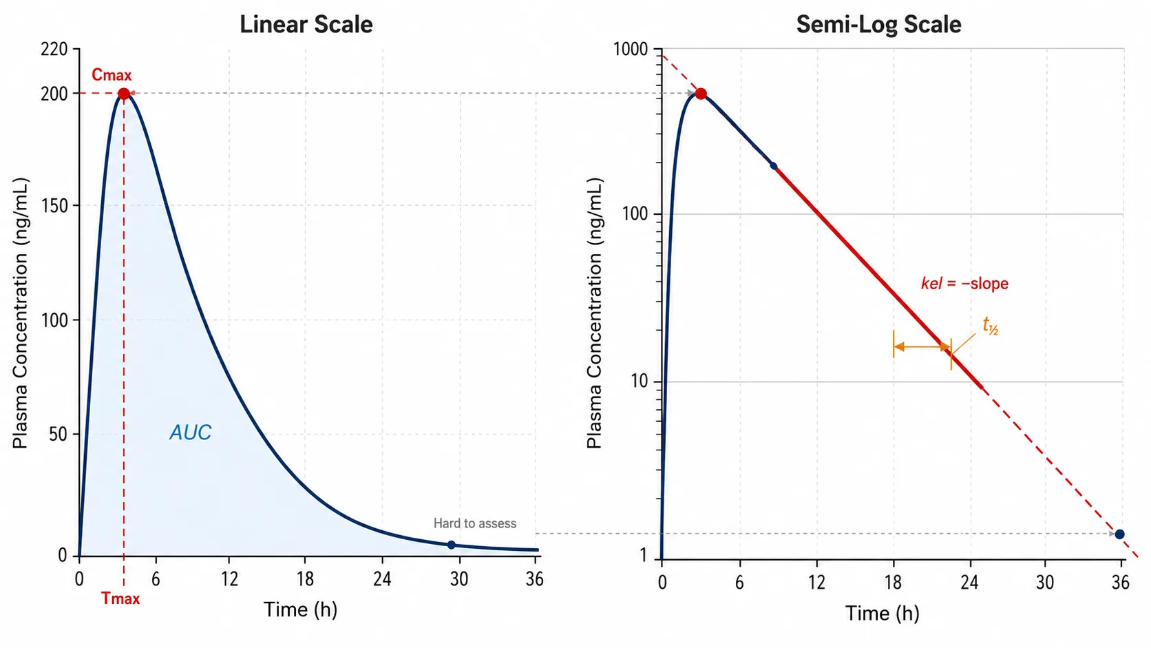 Figure 2: Side-by-side comparison — the same concentration-time data plotted on linear scale (left) and semi-log scale (right). Linear plot shows exponential decay curve with AUC shading. Semi-log plot shows the same data with a straight terminal line, kel slope annotation, and half-life illustrated as a horizontal segment showing concentration dropping by 50%. Cmax and Tmax marked on both plots.
Curve Shapes Tell the Story: Four Fundamental Profiles
The shape of a concentration-time curve is determined by the route of administration and the relationship between absorption and elimination rates. Recognizing the shape tells you what happened before any parameter is calculated.
Intravenous Bolus
No absorption phase. The curve starts at maximum concentration (C0 at t=0) and declines continuously. On semi-log, a one-compartment drug is a single straight line. A two-compartment drug shows a biphasic decline: a rapid distribution phase (α) followed by a slower elimination phase (β). The practical significance: IV data provides the only direct measurement of Vd and CL without the confounding effect of bioavailability (F). Every oral PK parameter that involves CL/F or Vd/F carries uncertainty from unknown F, which is why IV PK in preclinical species is essential for accurate compound ranking.
Oral Dosing (Immediate Release)
The classic three-phase profile: absorption, distribution, elimination. The peak reflects the balance between absorption and elimination. For drugs with ka >> kel (rapid absorption relative to elimination), the peak is sharp and the terminal phase directly reflects elimination. This is the normal case for most small-molecule drugs.
Oral Dosing (Flip-Flop Kinetics)
When absorption is slower than elimination (ka < kel), the terminal slope reflects absorption, not elimination. This is flip-flop kinetics. The curve after Cmax looks like a normal elimination phase, but the slope is actually ka, not kel. Flip-flop is common with sustained-release formulations, poorly soluble compounds, and intramuscular/subcutaneous depots. The diagnostic sign: the terminal half-life after oral dosing is longer than the IV half-life (when IV data is available). Without IV data, flip-flop can go unrecognized — and the reported "half-life" may actually be the absorption half-life, leading to incorrect dosing interval predictions. For methods requiring accurate terminal-phase quantification for flip-flop diagnosis, our LC-MS/MS method development and validation services include low-LLOQ optimization strategies for extended sampling durations.
IV Infusion
The concentration rises gradually toward a steady-state plateau (Css). At steady state, infusion rate = elimination rate. The curve shape is a hyperbolic approach: after one half-life, concentration reaches 50% of Css; after two half-lives, 75%; after four half-lives, ∼94%. The clinical relevance: loading doses (IV bolus at t=0 followed by infusion) are used to reach therapeutic concentrations immediately for drugs with long half-lives — the bolus fills the Vd, the infusion maintains it.
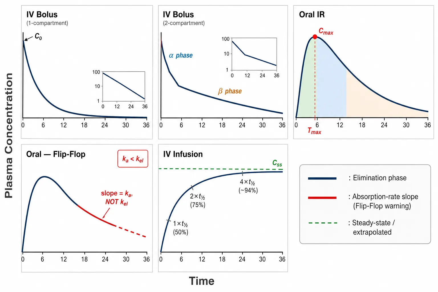 Figure 3: Four fundamental curve shapes — (A) IV bolus one-compartment: single exponential decay; (B) IV bolus two-compartment: biphasic decay with distribution and elimination phases labeled; (C) Oral immediate-release: classic three-phase with absorption, distribution, elimination; (D) Flip-flop kinetics: terminal slope labeled as "slope = ka, not kel — see text"; (E) IV infusion: hyperbolic approach to Css plateau. All panels share the same axes for comparison. A small annotation on each panel names the route and key diagnostic feature.
How to Estimate PK Parameters from the Curve
Cmax and Tmax — Direct Observation
Read Cmax as the highest measured concentration and Tmax as the time it occurs. No calculation. The reliability of both depends entirely on sampling density. A rule of thumb: at least two sampling points should fall between dosing and Tmax, one near Tmax, and at least three in the elimination phase. In practice, early development PK studies often under-sample the absorption phase, producing Cmax values that are lower than true Cmax and Tmax values that are later than true Tmax. When reviewing PK data: if Cmax occurs at the first sampling time point, the reported Cmax is a lower bound, not the true peak. Our LC-MS/MS single drug quantification services include sampling schedule consultation for first-in-human and preclinical PK studies.
AUC — Trapezoidal Rule
AUC is computed by dividing the concentration-time curve into vertical trapezoids between consecutive time points and summing their areas. The area of each trapezoid = (C₁ + C₂) / 2 × (t₂ − t₁). Software does the arithmetic, but the analyst decides two things: the trapezoidal rule (linear vs linear-up/log-down) and the terminal points used for extrapolation to infinity.
Linear trapezoidal: use linear interpolation between all consecutive points. Simple and standard for the absorption and distribution phases. Linear-up/log-down: use linear interpolation before Tmax (rising concentrations) and logarithmic interpolation after Tmax (declining concentrations). The linear-up/log-down method is generally preferred because logarithmic interpolation on the declining limb more accurately represents first-order elimination between sampled points — especially when sampling intervals are long in the terminal phase.
AUC₀→∞ = AUC₀→last + Clast / kel. The extrapolated tail (Clast / kel) should contribute less than 20% to AUC₀→∞. If it contributes more, the sampling duration was insufficient. For preclinical PK, extend sampling to at least 3-4 half-lives. For clinical studies, the FDA recommends sampling for at least 3 half-lives after Cmax.
Half-Life — Terminal Slope
On a semi-log plot, select the linear terminal points (typically the last 3-5 concentrations above LLOQ). Run linear regression of ln(concentration) vs time. kel = absolute value of the slope. t½ = ln(2) / kel.
The most consequential analytical decision in NCA is which points to include in the terminal slope regression. Common errors: (1) including distribution-phase points — this produces a steeper slope and shorter half-life; (2) including concentrations near the LLOQ with high analytical variability — one noisy terminal point can shift kel by 15-30%; (3) using too few points — two points always produce perfect r² but zero diagnostic value. Our full and partial method validation services include precision profiling at the LLOQ to ensure terminal-phase concentrations are analytically reliable for slope estimation.
Clearance and Vd — Derived from AUC
After IV dosing: CL = Dose / AUC₀→∞. Vd = Dose / (kel × AUC₀→∞) = CL / kel. After oral dosing: CL/F = Dose / AUC₀→∞ and Vd/F = Dose / (kel × AUC₀→∞). The "/F" notation is a constant reminder that oral CL and Vd estimates contain unknown bioavailability — they are apparent values. Comparing oral CL/F across compounds without IV CL data is comparing a hybrid parameter (clearance divided by an unknown).
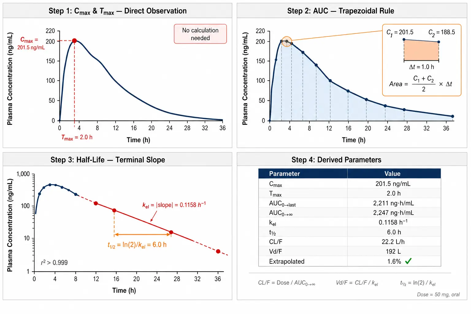 Figure 4: Step-by-step parameter estimation visual guide — a single oral concentration-time curve with (A) Cmax and Tmax read directly as dashed horizontal/vertical lines to the peak, (B) AUC shown as stacked trapezoids with one trapezoid zoomed to show the area formula, (C) terminal phase on semi-log inset with the 3 regression points highlighted and kel = |slope| labeled, (D) summary box showing all derived parameters with formulas: t½ = 0.693/kel, CL/F = Dose/AUC, Vd/F = CL/kel.
Curve Patterns That Demand Attention
Some curves contain features that are easy to miss on a cursory glance but have important PK implications.
Double Peaks
Two distinct Cmax values separated by a concentration trough. Most common cause: enterohepatic recirculation — drug excreted in bile is reabsorbed in the intestine, producing a second absorption event hours after the first. Other causes: gastric emptying variability (one fraction empties early, another later) or site-specific absorption along the intestine (two absorption windows with different permeability). Double peaks are physiologically real — do not dismiss them as assay variability. For enterohepatic recirculation, bile duct-cannulated animal studies can confirm the mechanism. From the bioanalytical perspective, double-peak profiles require adequate late-time sampling to fully capture the second peak's AUC contribution — truncating sampling at the trough between peaks underestimates total exposure.
Delayed Absorption
A prolonged lag time followed by normal absorption. Common with food-effect studies where gastric emptying is delayed, with enteric-coated formulations, or with drugs that are substrates for intestinal efflux transporters (P-gp, BCRP) that must be saturated before absorption proceeds. The diagnostic feature: Tmax shifts right by 2-6 hours with no change in Cmax or AUC. Delayed Tmax without reduced AUC is not a bioavailability problem — it is a rate problem that may or may not matter depending on the therapeutic indication.
Unexpected Terminal Rise
Concentration increases during what should be the elimination phase. Usually a bioanalytical artifact: loss of IS response at late time points due to differential stability, or carryover from a preceding high-concentration sample. Rule out analytical causes before attributing to physiology. If real, possible explanations include: metabolite back-conversion to parent (e.g., acyl glucuronide hydrolysis at physiological pH), saturable tissue binding with late release, or circadian variation in clearance. When metabolite profiling is needed to distinguish these mechanisms, our high-resolution metabolite quantification services provide simultaneous parent-metabolite profiling to identify metabolite-to-parent back-conversion.
Sampling Strategy: Getting the Curve Right Before the Assay
The best LC-MS/MS method cannot rescue a poorly sampled concentration-time curve. Bioanalytical scientists have an opportunity — and a responsibility — to provide input on PK study design before samples arrive.
Number of Time Points
For oral PK, 8-12 time points are standard for a single-dose profile. Preclinical: predose, 0.25, 0.5, 1, 2, 4, 6, 8, 12, 24 h is a common rat PK schedule. Clinical: add a 0.5 h and a 36 or 48 h point for drugs with t½ > 8 h. The cost of an extra time point is trivial compared to the cost of an uninterpretable curve.
Absorption Phase Density
Two to three points before Tmax. If the expected Tmax is unknown (first-in-human), sample at 0.25, 0.5, 1, 1.5, 2, and 3 h to bracket the range of possible absorption rates. Once Tmax is established from single-dose data, subsequent studies can reduce early sampling.
Terminal Phase Duration
Sample for at least 3 half-lives after the last expected Cmax. If half-life is unknown from prior data, extend sampling to 72 or 96 h for first-in-human studies. The practical limit: concentrations below 5% of Cmax approach the assay LLOQ, and analytical variability at these levels can distort the terminal slope. For comprehensive PK study support covering sampling design and validated quantification from early preclinical through clinical phases, our LC-MS/MS plasma and serum drug quantification services support full-profile PK with calibration ranges tailored to expected in vivo concentrations.
From Raw Data to Curve to Parameters: A Practical Walkthrough
Consider a single oral 50 mg dose in a healthy volunteer. Plasma samples were collected at 0, 0.5, 1, 1.5, 2, 3, 4, 6, 8, 12, 24, and 36 h, processed by PPT with acetonitrile containing a stable isotope-labeled internal standard (SIL-IS), and analyzed by LC-MS/MS (LLOQ = 1.0 ng/mL). Proper IS selection is the single largest factor in method precision for PK studies — a well-matched SIL-IS corrects for extraction variability, matrix effects, and ion source fluctuation simultaneously. Our internal standard selection and optimization services provide SIL-IS sourcing, feasibility testing, and matrix-specific performance evaluation for preclinical and clinical PK assays.
The concentration data: 0, 127.7, 180.9, 199.2, 201.5, 188.5, 170.0, 135.4, 107.5, 67.7, 16.9, 4.2 ng/mL at each time point.
| Time (h) |
Plasma Concentration (ng/mL) |
| 0.0 |
0.0 |
| 0.5 |
127.7 |
| 1.0 |
180.9 |
| 1.5 |
199.2 |
| 2.0 |
201.5 ← Cmax |
| 3.0 |
188.5 |
| 4.0 |
170.0 |
| 6.0 |
135.4 |
| 8.0 |
107.5 |
| 12.0 |
67.7 |
| 24.0 |
16.9 |
| 36.0 |
4.2 |
Step 1 — Plot the curve. On linear scale, the absorption phase rises to a clear Cmax of 201.5 ng/mL at Tmax = 2.0 h, followed by a curved decline that approaches zero asymptotically. No double peaks. No outliers.
Step 2 — Plot on semi-log. The terminal phase (8, 12, 24, 36 h) is clearly linear. Select these four points for the terminal regression.
Step 3 — Calculate kel. Linear regression of ln(concentration) vs time for the last 4 points: slope = −0.1158 h⁻¹. r² > 0.999 — the terminal points are highly consistent. t½ = 0.693 / 0.1158 = 6.0 h.
Step 4 — Calculate AUC. AUC₀→last by linear trapezoidal: 2,211 ng·h/mL. Extrapolated tail: Clast / kel = 4.2 / 0.1158 = 36.3 ng·h/mL. AUC₀→∞ = 2,211 + 36.3 = 2,247 ng·h/mL. Extrapolated fraction: 1.6% — well within the 20% threshold, and the 36-h sampling duration (6 half-lives) provided excellent terminal-phase coverage.
Step 5 — Calculate CL/F and Vd/F. CL/F = 50,000 µg / 2,247 ng·h/mL = 22.2 L/h. Vd/F = CL/F / kel = 22.2 / 0.1158 = 192 L. The apparent volume far exceeds total body water (∼42 L), indicating extensive tissue distribution — consistent with a lipophilic basic drug.
Step 6 — Interpret. Half-life of 6.0 h supports twice-daily dosing (every ∼2 half-lives). CL/F of 22.2 L/h is low-to-moderate — the drug is not a high-clearance compound (hepatic blood flow ∼90 L/h). The sampling scheme, with 12 time points over 36 h (6 half-lives), provided excellent terminal phase definition. The extrapolated fraction of 1.6% means the reported AUC₀→∞ is almost entirely from observed data, not extrapolation — the strongest possible foundation for CL/F and Vd/F estimation.
This walkthrough illustrates a key principle: the curve dictates which parameters you can reliably estimate, not the other way around. If the same data had been truncated at 12 h (last concentration = 67.7 ng/mL), the extrapolated fraction would rise substantially, kel would shift because only 3 terminal points would be available (6, 8, 12 h), and CL/F and Vd/F would change accordingly. The curve is the evidence — parameters are summaries of it.
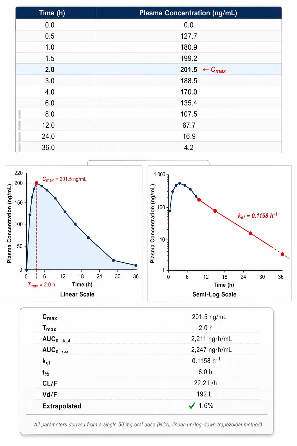 Figure 5: Complete data walkthrough in a single multi-panel figure. (A) The concentration-time data table (12 time points, concentrations from 0 to 201.5 ng/mL). (B) Linear-scale curve with Cmax and Tmax marked. (C) Semi-log curve with the 4 terminal regression points highlighted and kel slope drawn. (D) Summary parameter table: Cmax = 201.5 ng/mL, Tmax = 2.0 h, AUC₀→∞ = 2,247 ng·h/mL, t½ = 6.0 h, CL/F = 22.2 L/h, Vd/F = 192 L, Extrapolated = 1.6%.
Frequently Asked Questions
What is the most common mistake when reading a concentration-time curve?
Trusting parameters without looking at the curve first. Before accepting any PK report, look at the semi-log plot. Does the terminal phase contain at least 3 points? Is the extrapolated AUC under 20%? Is Cmax bracketed by sampling points (not at the first or last point)? Are there any unexpected bumps, rises, or flat regions? Software will generate parameters from nearly any data — the curve reveals whether those parameters are trustworthy. A second common mistake: using a linear scale for terminal-phase assessment. First-order elimination that looks clean on a linear plot can reveal itself as biphasic or distorted on semi-log.
When should I suspect flip-flop kinetics?
Suspect flip-flop when: (1) the terminal half-life after oral dosing is longer than the IV half-life for the same compound; (2) the terminal slope after an immediate-release oral dose is unusually shallow relative to what is expected for this chemical class; (3) Cmax is low and Tmax is late (>4 h) for a compound with good permeability. Confirm by comparing oral and IV half-lives when IV data exists. Without IV data, the distinction cannot be made definitively from a single oral curve. For sustained-release formulations, flip-flop is the intended design — the terminal slope is absorption rate and should be slower than the elimination rate from an immediate-release reference.
What is the difference between AUC₀→last and AUC₀→∞, and when does the distinction matter?
AUC₀→last is the trapezoidal area from time zero to the last measurable concentration — purely from observed data, no extrapolation. AUC₀→∞ adds the extrapolated tail (Clast / kel). The distinction matters most when: (1) the sampling duration is short relative to half-life (extrapolated fraction > 20%) — in this case, AUC₀→∞ is unreliable and AUC₀→last should be reported instead for that subject; (2) comparing studies with different sampling durations (one stops at 24 h, the other at 48 h) — AUC₀→last will differ systematically even if the drug behaved identically; (3) bioequivalence studies, where regulatory authorities require AUC₀→t (AUC to the last common time point across subjects) rather than AUC₀→∞ when the terminal phase is poorly defined. For a full discussion of how AUC is derived from validated concentration data and the bioanalytical factors that affect AUC accuracy, see our guide on plasma drug concentration fundamentals.
Why do some drugs show double peaks?
Enterohepatic recirculation is the most common cause — drug is absorbed, glucuronidated in the liver, excreted in bile, and the glucuronide is hydrolyzed back to parent drug by gut bacteria in the colon, followed by reabsorption. This produces a second peak typically 6-12 h after the first. Less common causes include: gastric emptying variability (a fraction of the dose is retained in the stomach and empties later), site-specific intestinal absorption, or metabolite back-conversion in plasma. Distinguishing these mechanisms requires additional experiments: bile duct-cannulated animals for enterohepatic recirculation, or metabolite profiling to detect conjugate hydrolysis. For matrix-matched bioanalytical support with challenging sample types, our bioanalysis services for challenging compounds and complex matrices cover plasma, bile, and tissue homogenate matrices.
How many subjects are needed to characterize a concentration-time curve?
For preclinical PK, N = 3 per time point (rodent destructive sampling, composite profile) or N = 3-4 serial sampling (large animals). For clinical single-dose PK, N = 6-12 healthy volunteers is typical for initial characterization. For bioequivalence studies, N is determined by power analysis based on intra-subject CV of AUC and Cmax — typically 18-48 subjects for a standard two-period crossover. The key variable is intra-subject variability, not inter-subject variability, because BE studies use crossover designs. If intra-subject CV exceeds 30% for AUC or Cmax, the drug is classified as highly variable and the reference-scaled average bioequivalence (RSABE) approach may apply per FDA guidance.
Can I estimate PK parameters without IV data?
Yes, but with limitations. After oral dosing, you can estimate Cmax, Tmax, t½, and AUC without IV data. However, CL/F and Vd/F are apparent values — they include the unknown bioavailability F. You cannot determine whether a low oral AUC is due to high clearance or low bioavailability without an IV reference. This is why preclinical programs routinely include both IV and oral arms in definitive PK studies: the IV leg provides CL and Vd directly, the oral leg provides Cmax, Tmax, and F. Together, they provide the complete picture. For preclinical programs needing both IV and oral PK support, our custom LC-MS/MS method development services provide matched IV/oral methods with cross-matrix validation across plasma from multiple preclinical species.
References
- Krishna R, Yu R. An ABC of PK/PD. Open Education Alberta. 2023. CC BY 4.0.
- Benet LZ, Sodhi JK. Simplifying pharmacokinetics, applying it to drug and dosage form development, and making drug dosage decisions in clinical medicine: the adaptation of Kirchhoff's laws from physics. The AAPS Journal. 2025;27:53.
- U.S. Food and Drug Administration. Bioavailability and Bioequivalence Studies Submitted in NDAs or INDs — General Considerations. FDA Guidance for Industry; 2019.
- European Medicines Agency. ICH Guideline M10 on Bioanalytical Method Validation and Study Sample Analysis. EMA/CHMP/ICH/172948/2019; 2022.
- Liu G, Brooks L, Canty J, Lu D, Jin JY, Lu J. Deep-NCA: A deep learning methodology for performing noncompartmental analysis of pharmacokinetic data. CPT: Pharmacometrics & Systems Pharmacology. 2024;13(5):870-879. CC BY 4.0.
- Chen X, Nyberg HB, Donnelly M, Zhao L, Fang L, Karlsson MO, Hooker AC. Development and comparison of model-integrated evidence approaches for bioequivalence studies with pharmacokinetic end points. CPT: Pharmacometrics & Systems Pharmacology. 2024;13(10):1734-1747. CC BY 4.0.
- Myler H, Evans C, Garofolo F, et al. ICH M10 Bioanalytical Method Validation Guideline — 1 Year Later. The AAPS Journal. 2024;26:103. CC BY 4.0.
- Bacila CI, Macavei BM, Cornea M, et al. UHPLC-MS/MS for antipsychotic drug monitoring: a systematic review of clinical and analytical performance. Journal of Clinical Medicine. 2025;14(21):7544. CC BY 4.0.
Disclaimer: All services and resources mentioned on this site are for research use only (RUO) and are not intended for diagnostic, therapeutic, or clinical applications.
Related Services