Tissue Drug Quantification by LC-MS/MS: From Solid Tissue to Validated Concentration Data

Most drug development programs measure drug concentrations in plasma — because plasma is convenient, because regulatory guidance is built around plasma, and because plasma concentration is the input to the pharmacokinetic parameters that drive dose selection. But for many drug target classes — oncology agents targeting tumor kinases, CNS drugs intended for brain parenchyma, antivirals whose replication site is in the liver — the plasma concentration is not the concentration at the site of action. Tissue drug concentration determines target engagement, predicts efficacy, and explains toxicities that plasma exposure cannot. Measuring it correctly requires solving problems that do not exist in plasma bioanalysis: no authentic blank matrix for calibration, a two-stage recovery process (homogenization then extraction), multi-source ion suppression far exceeding plasma levels, and an incurred sample reanalysis (ISR) landscape complicated by tissue heterogeneity. This article provides the practical workflow — from homogenized tissue to validated concentration data — that bioanalytical scientists need but that no CRO has integrated into a single guide. For the homogenization methods that precede the quantification steps described here, see our article on tissue homogenization methods comparison, which covers bead beating, rotor-stator, and enzymatic digestion method selection. Our tissue and cell lysate drug quantification services provide validated workflows from homogenization through LC-MS/MS analysis for all major organ types.

Why Tissue Quantification Is Fundamentally Different from Plasma

Plasma bioanalysis starts with a liquid sample that can be pipetted, spiked, and extracted with well-characterized matrix effects. Tissue bioanalysis starts with a solid organ piece that must be physically disrupted before any downstream step, with drug distributed heterogeneously across anatomical compartments, and without the authentic blank matrix that is the foundation of calibrator and QC preparation in plasma methods. These three differences — solid state, heterogeneous distribution, absent blank matrix — define the tissue quantification problem.

The first difference, the solid state, is addressed by homogenization (covered in the A10 article). The output of homogenization is a slurry — tissue homogenate — that can be pipetted and extracted like plasma. But this homogenate is not plasma. It contains cytosolic proteins at milligram-per-milliliter concentrations, phospholipids at 5- to 50-fold higher abundance than plasma, heme iron-porphyrin from residual blood, and DNA/RNA polyanions from lysed nuclei. Each of these components contributes to ion suppression or enhancement in the LC-MS/MS source, and the mix varies by tissue type, by perfusion status at collection, and by homogenization method.

The second difference, heterogeneous drug distribution, means the concentration measured from one tissue sub-sample may not represent the whole organ. Liver drug concentration differs between portal and central lobular regions. Kidney cortex and medulla drug concentrations can differ by several-fold. Brain gray matter and white matter are pharmacokinetically distinct compartments. The bioanalytical method must account for this heterogeneity through standardized sampling, and the ISR assessment must acknowledge it.

The third difference — the absence of authentic blank tissue — is the defining analytical challenge. In plasma bioanalysis, calibration standards and QCs are prepared by spiking reference standard into blank (drug-free) plasma from the same species, often the same matrix lot. Blank tissue from untreated animals exists, but spiking drug onto or into intact tissue does not replicate the in vivo drug distribution state — the drug sits on surfaces and in extracellular spaces, not inside cells, not bound to intracellular proteins. The recovery measured from such a preparation reflects extraction from the homogenate, not recovery from the true incurred state. Every calibration approach for tissue is therefore a compromise, and selecting the right compromise is the most consequential method development decision. For bioanalytical method development that addresses tissue-specific calibration challenges, our bioanalytical method development and validation services include systematic evaluation of surrogate matrix suitability and calibration strategy for each tissue type.

The Calibration Strategy: Solving the "No Blank Tissue" Problem

Because authentic blank tissue matrix cannot be prepared in a way that replicates incurred drug distribution, every tissue calibration approach uses a substitute. Three strategies are available, and the choice depends on sample throughput, regulatory context, and the tissue type.

Strategy 1 — Surrogate matrix calibration. This is the most practical and widely used approach. Calibration standards are prepared in a surrogate matrix — typically plasma, 4-5% bovine serum albumin (BSA) in PBS, or a solvent mixture such as 50:50 methanol:water. The homogenate from an incurred tissue sample is extracted alongside these surrogate-matrix calibrators, and the resulting concentration is corrected for any systematic difference between surrogate and authentic tissue matrix. The critical validation experiment is parallelism: spike the same concentration of analyte into surrogate matrix and into tissue homogenate from a pooled incurred sample (which already contains drug), measure the response at three or more concentrations, and compare. Acceptance criteria: IS-normalized matrix factor 0.85-1.15 for each concentration level, and the slope ratio of the tissue homogenate response-versus-concentration line to the surrogate matrix line should be 0.90-1.10. If parallelism passes, surrogate matrix calibration is valid. If parallelism fails — the surrogate and tissue responses diverge — switch to standard addition.

The parallelism experiment deserves careful attention because it is frequently performed incorrectly. The pooled incurred homogenate must come from multiple animals to average out individual variability. The spiked concentrations must span the expected study sample range — parallelism at low concentration does not guarantee parallelism at high concentration, and vice versa. And the experiment must be repeated if the tissue type changes; parallelism in liver homogenate does not establish parallelism in lung. Ho and Gao (2015) provide a comprehensive framework for surrogate matrix validation in tissue analysis, including the four-method comparison (calibration curve slopes, QC accuracy, recovery, and matrix effect) that regulatory reviewers expect. For laboratories establishing tissue methods for the first time, our method validation services include full surrogate matrix qualification with the four-method comparison recommended by Ho and Gao (2015).

Strategy 2 — Standard addition. The incurred tissue homogenate is divided into multiple aliquots (typically 5-6). Increasing known amounts of drug are spiked into each aliquot. A regression of response versus spike amount is constructed, and the x-intercept (extrapolated backward to zero response) gives the original homogenate concentration. This method is self-calibrating — it requires no external calibration curve and no blank or surrogate matrix. Its limitation is throughput: each sample requires its own multi-point calibration, consuming significant homogenate volume and instrument time. Standard addition is best reserved for low-N critical samples, confirmatory reanalysis when surrogate matrix parallelism is borderline, and method cross-validation between tissue types.

Strategy 3 — External calibration with matrix factor correction. Calibration standards are prepared in a simple solvent (no matrix). The matrix effect is measured separately — typically by post-column infusion of analyte into extracted tissue homogenate — and a correction factor is applied to the solvent-calibration result. This is the fastest approach but carries the highest risk: matrix effects in tissue are not constant across the chromatographic run, and a single correction factor may not adequately correct for suppression that co-elutes with the analyte. This strategy is acceptable for discovery-stage screening but is difficult to defend in a regulated bioanalysis context.

The decision tree: for regulated studies with sufficient sample volume, surrogate matrix calibration with validated parallelism is the primary recommendation. For discovery screening, external calibration with a matrix factor check may suffice. For critical samples or failed parallelism, use standard addition. For a comprehensive tissue quantification workflow that includes calibration strategy selection and validation, our custom LC-MS/MS method development services design and validate tissue-specific calibration approaches for each matrix type.

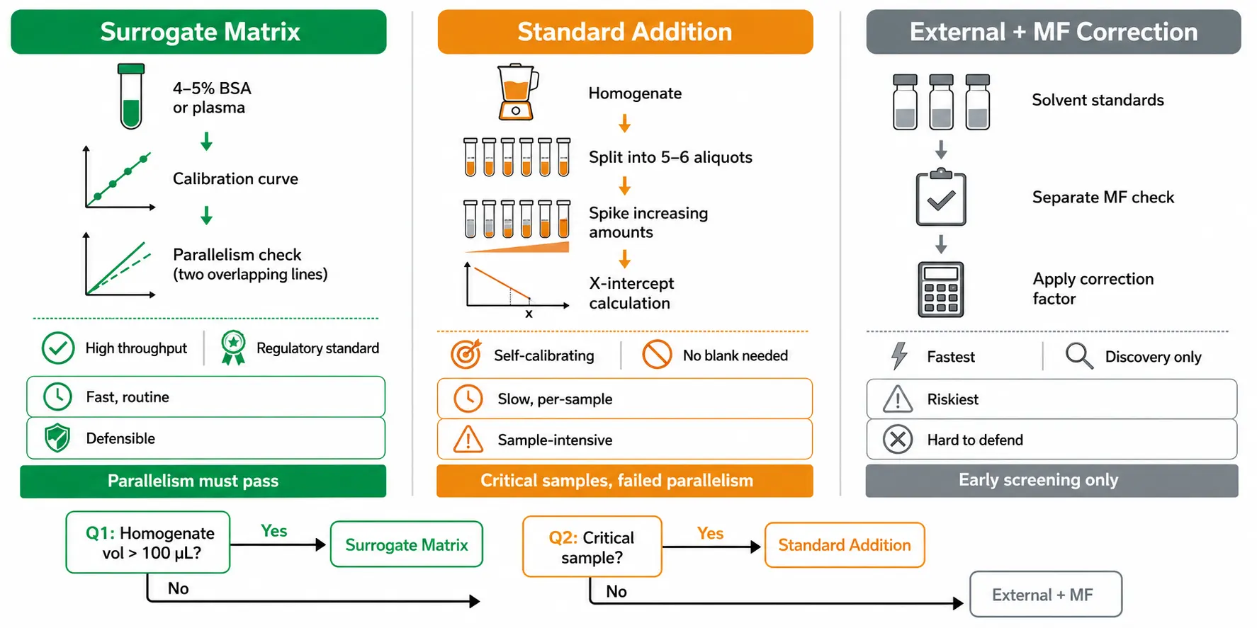Figure 1: Calibration strategy decision tree. Three columns representing the three strategies: Surrogate Matrix (left, green accent), Standard Addition (center, amber accent), External + MF Correction (right, gray accent). Each column shows: (1) workflow icon sequence, (2) throughput rating (high/medium/low), (3) regulatory defensibility rating, and (4) "Best when:" usage-context line. Bottom: decision-tree arrows — "Homogenate volume > 100 µL?" → yes → Surrogate Matrix; no → "Critical sample?" → yes → Standard Addition; no → External + MF. Clean white background, sans-serif, minimal text.

Tissue-Specific Matrix Effects: Why Tissue Is Harder Than Plasma

Plasma matrix effects in LC-MS/MS are dominated by phospholipids — primarily phosphatidylcholines and lysophosphatidylcholines that co-elute in the 2-5 minute retention time window under reversed-phase conditions. Phospholipid removal strategies (PPT with cold acetonitrile, hybrid SPE, HILIC) are well established for plasma. Tissue homogenates present a more complex matrix effect landscape driven by multiple compound classes at concentrations far exceeding plasma levels.

Phospholipids in tissue homogenates are present at 5- to 50-fold higher abundance than in plasma, with brain and adipose tissue being the worst offenders. The phospholipid composition also differs by tissue type: brain is enriched in phosphatidylserine and phosphatidylethanolamine; liver contains high phosphatidylcholine; adipose contains triglycerides that form a floating lipid layer in aqueous homogenate. A protein precipitation step that adequately removes plasma phospholipids may be insufficient for tissue homogenate.

Heme iron-porphyrin from residual blood in the tissue introduces a chemically distinct class of interferent. Heme produces strong UV absorption at 400 nm (Soret band) and can form non-covalent adducts with basic drugs via π-π stacking with the porphyrin ring system. These adducts suppress ionization in electrospray by competing for surface charge at the droplet interface. Perfusing the tissue with saline at collection to remove residual blood reduces heme interference but also risks washing out drug from the extracellular compartment — the perfusion decision must balance analytical cleanliness against recovery accuracy.

Cytosolic structural proteins — actin, tubulin, myosin — are present in tissue homogenate at mg/mL concentrations. During protein precipitation with organic solvent, these proteins denature and precipitate, but incomplete precipitation leaves residual soluble peptides that co-elute broadly across the chromatogram. These peptides contribute to a general elevation of baseline and can cause variable ion suppression across the analyte retention time window.

DNA and RNA polyanionic backbones, released from nuclei lysed during homogenization, present a tissue-specific interference mechanism not encountered in plasma. The phosphate backbone carries a high negative charge density that can form electrostatic adducts with basic (positively charged) drugs, particularly amines with pKa > 8. These adducts may be stable enough to survive the extraction and co-elute with the analyte, producing either suppression or enhancement depending on the adduct's ionization efficiency relative to the free drug.

The presence of multiple interference classes with different chemical properties, each varying by tissue type and homogenization method, means that a one-size-fits-all matrix effect mitigation strategy is unlikely to succeed. Method development must characterize the specific suppression profile for each tissue type in the study. A post-column infusion experiment — infusing a constant stream of analyte into the LC effluent while injecting extracted tissue homogenate — identifies the retention time zones where suppression or enhancement occurs. If the analyte elutes in a suppression zone, modify the chromatography to shift the analyte into a clean region, or increase sample cleanup (switch from PPT to SPE, or add a hexane defatting step before extraction). For tissue types known to produce complex matrix effects, our complex biological matrices analysis services provide tissue-specific matrix effect profiling and cleanup optimization.

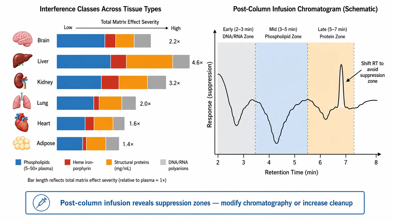Figure 2: Tissue-type matrix effect comparison. Six horizontal bars (brain, liver, kidney, lung, heart, adipose), each showing relative abundance of four interference classes: phospholipids (blue), heme (red), structural proteins (amber), DNA/RNA (gray). Bar width proportional to abundance. Right side: schematic chromatogram with shaded suppression zones mapped to each interference class. Bottom text: "Post-column infusion reveals suppression zones — shift analyte retention time or increase cleanup." Clean white background.

The Two-Stage Recovery Problem: Why Most Recovery Measurements Are Incomplete

In plasma bioanalysis, recovery is a single-stage measurement: spike drug into blank plasma, extract, and compare the response to a reference solution spiked post-extraction. The measurement captures extraction recovery — how much drug the sample preparation method retrieves from the matrix.

In tissue bioanalysis, recovery has two sequential stages. Stage 1 is homogenization recovery — how completely the homogenization method releases drug from intact tissue cells and structural proteins into the liquid homogenate. Stage 2 is extraction recovery — how much of the drug in the homogenate is recovered by the subsequent PPT, LLE, or SPE step. Total method recovery is the product: total recovery = homogenization efficiency × extraction recovery.

A method that achieves 95% extraction recovery but only 60% homogenization efficiency delivers 57% total recovery — and the 60% homogenization efficiency means 40% of the drug in the tissue was never available for extraction. This is not a hypothetical scenario. Liang et al. (2011) demonstrated that rotor-stator homogenization of mouse liver produces 20-30 μm residual particles that contain unreleased drug, and Qin et al. (2015) showed that bead beating alone recovers below 50% of drug from lung and skin tissue relative to collagenase-assisted homogenization.

The problem is that most method development protocols measure only extraction recovery — spiking drug into homogenate and measuring retrieval — without measuring homogenization efficiency. The resulting recovery number overestimates true method recovery by an unknown margin. The fix: during method development, compare drug concentrations obtained by the planned homogenization method against those obtained by a maximally disruptive reference method — collagenase digestion followed by extended bead beating, or cryogenic milling in liquid nitrogen. If the planned method yields lower concentrations than the reference method for the same tissue, it is leaving drug behind. The reference method need not be practical for routine use (collagenase digestion of hundreds of samples is too slow); it serves as the benchmark.

A second validation approach is to spike drug into naive tissue, allow penetration (incubate at 37°C for 1 hour), then subject the tissue to the planned homogenization and extraction workflow. While this does not replicate in vivo distribution, it does test whether the method can recover drug that has penetrated into the tissue interior — a more stringent test than spiking drug onto the homogenate surface. If recovery from spiked intact tissue matches recovery from spiked homogenate, homogenization is not a bottleneck. If spiked intact tissue recovery is lower, homogenization is incomplete. For tissue method development including the two-stage recovery assessment, our sample preparation and processing services include homogenization efficiency evaluation against reference methods for each tissue type.

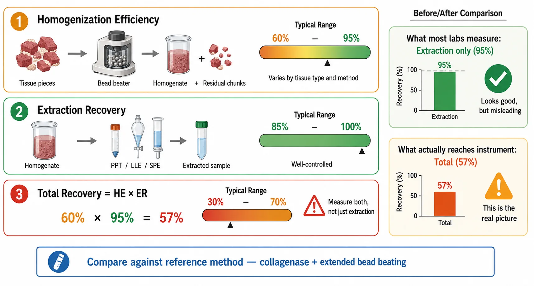Figure 3: Two-stage recovery concept diagram. Left bar: "Homogenization Efficiency" (60-95%, varies by tissue) — icon of tissue pieces breaking apart. Center bar: "Extraction Recovery" (85-100%) — icon of liquid-liquid partition. Right bar: "Total Recovery" = product of two — with worked example: 95% extraction × 60% homogenization = 57% total. Bottom warning: "Measure both, or you're seeing half the picture." Clean white background, color gradient from amber (low) to green (high).

Sample Preparation for Tissue Homogenates

Tissue homogenate is a more complex sample matrix than plasma, and the sample preparation method must address the additional interference classes while maintaining acceptable throughput. The three standard techniques — protein precipitation (PPT), liquid-liquid extraction (LLE), and solid-phase extraction (SPE) — each have tissue-specific considerations.

Protein precipitation with acetonitrile or methanol (typically 3:1 v/v organic:homogenate) is the fastest method and is adequate for tissues with moderate matrix effect profiles — liver, kidney, and brain homogenates at 1:4 or higher dilution. For tissues with high lipid content (adipose, brain), pre-cool the homogenate and organic solvent to 4°C — cold PPT precipitates lipids more efficiently than room-temperature PPT, reducing phospholipid carryover into the supernatant. After vortex mixing and centrifugation (14,000 × g, 10 minutes, 4°C), the supernatant is typically diluted 1:1 with water before injection to improve peak shape for early-eluting analytes.

Liquid-liquid extraction with methyl tert-butyl ether (MTBE) or hexane:ethyl acetate mixtures provides cleaner extracts than PPT because lipids partition into the organic phase while most drug molecules (unless highly lipophilic, logD > 4) remain in the aqueous phase. This is the reverse of conventional LLE logic: in tissue homogenate LLE, the organic solvent removes lipids (discarded), and the aqueous phase containing the drug is retained for analysis. MTBE is preferred over hexane because it forms the upper organic layer, simplifying aqueous phase recovery. This approach is particularly effective for adipose tissue homogenates.

Solid-phase extraction provides the cleanest extracts and is recommended for tissues with severe matrix effects or when the analyte is present at low concentrations requiring maximal sensitivity. Mixed-mode SPE (e.g., Waters Oasis MCX for basic drugs, MAX for acidic drugs) provides orthogonal retention: reversed-phase retention of the drug followed by ion-exchange wash and elution, removing both neutral lipids (washed off in the organic step) and charged interferences (separated by the ion-exchange step). The trade-off is throughput — a 96-well SPE plate adds 20-30 minutes to the sample preparation protocol relative to PPT.

For tissues with high blood content (spleen, highly perfused liver), an optional pre-wash step may help: homogenize tissue in buffer, centrifuge briefly (1,000 × g, 2 minutes) to pellet tissue fragments, discard supernatant containing blood components, then re-suspend the pellet in fresh buffer for homogenization. This reduces heme interference but carries the risk of discarding drug in the blood fraction — validate by comparing concentration with and without the pre-wash for incurred tissue samples. For tissue extraction optimization across diverse tissue types, our single drug quantification services provide tissue-specific sample preparation protocols developed against matrix-matched calibration standards.

Method Validation for Tissue Assays: What Changes from Plasma

ICH M10 provides the framework for bioanalytical method validation, but tissue assays require tissue-specific additions and modifications to each validation parameter. The core parameters — accuracy, precision, selectivity, calibration model, matrix effect, dilution integrity, stability — all apply, but the execution differs when authentic blank matrix is unavailable.

Accuracy and precision are assessed using QCs prepared in surrogate matrix at a minimum of four concentration levels (LLOQ, low, mid, high), analyzed across at least three independent runs. Acceptance criteria — ±15% (±20% at LLOQ) for accuracy, ≤15% (≤20% at LLOQ) for precision — are identical to plasma methods. However, tissue method accuracy carries an irreducible uncertainty: the surrogate matrix QCs do not replicate the true incurred drug distribution state. The parallelism experiment (described in the Calibration Strategy section) is the evidence that this uncertainty is acceptably small.

Selectivity requires demonstrating that the tissue homogenate from at least six individual sources (each from a different naive animal of the relevant species and strain) produces no interfering peaks at the analyte retention time exceeding 20% of the LLOQ response. For large-animal studies where six individual sources may be impractical, use the available number with scientific justification. A separate selectivity assessment should evaluate whether homogenization method components — bead material leachables, collagenase residues, buffer components — produce interference. Analyze a matrix blank (homogenization buffer processed through the full homogenization procedure without tissue) alongside the tissue blanks.

Matrix effect must be assessed in at least six lots of tissue homogenate (six different naive animals). Calculate the IS-normalized matrix factor for each lot at low and high QC concentrations. The CV of the IS-normalized MF across the six lots should be ≤15%. If the CV exceeds 15%, the matrix effect is lot-dependent and the surrogate matrix approach may be unreliable — consider standard addition. For cross-tissue methods (same analyte, multiple organs), matrix effect must be assessed separately for each tissue type.

Tissue-specific validation additions: (a) Tissue weight linearity — prepare QC samples at 25%, 50%, 100%, and 200% of the nominal tissue weight (e.g., 0.25, 0.5, 1.0, and 2.0 g), keeping buffer volume constant. The back-calculated concentration should be independent of tissue weight (≤15% difference across the range). Deviation at high tissue weight indicates incomplete homogenization — the buffer is saturated with tissue solids and cannot fully disrupt the matrix. Deviation at low tissue weight indicates inadequate sensitivity. (b) Homogenization time course — homogenize replicate tissue samples for 2, 4, 6, 8, and 12 minutes. Plot measured concentration versus homogenization time; the concentration should plateau at the time required for complete disruption. Use the time at which concentration reaches 90% of the plateau value. (c) Regional variability — for large organs (liver, kidney, brain), compare measured concentrations from different anatomical sub-regions (left vs right lobe, cortex vs medulla). The CV across regions should be ≤20%; higher CV indicates that sub-sampling is introducing bias and the sampling protocol must be standardized. For tissue method validation that incorporates these tissue-specific parameters, our method validation services cover the full ICH M10 parameter set with tissue-specific additions.

Homogenate stability is distinct from tissue stability and must be assessed separately. Homogenization releases lysosomal enzymes — proteases, nucleases, lipases — from their compartmentalized intracellular locations. These enzymes can degrade the analyte in the homogenate at rates far exceeding degradation in intact tissue. Assess homogenate stability by re-analyzing QCs in homogenate at 0, 2, 4, 8, and 24 hours after preparation. If analyte degradation exceeds 15% within the expected batch processing time, add stabilizers (protease inhibitor cocktail, PMSF, EDTA) to the homogenization buffer, or reduce batch size to shorten homogenate-to-extraction time.

Dilution integrity is especially important for tissue assays because tissue drug concentrations frequently exceed plasma concentrations by 10- to 100-fold for drugs with high tissue distribution (Kp > 10). Prepare a QC at 5-10× the ULOQ (in surrogate matrix), then dilute 10-fold and 100-fold with surrogate matrix (not solvent — solvent dilution changes the matrix composition and may alter the matrix effect). The diluted result should be within ±15% of the nominal value after accounting for the dilution factor. Validate at the maximum dilution expected in study sample analysis.

Incurred Sample Reanalysis (ISR) for tissue has a fundamental difference from plasma ISR. In plasma ISR, the reanalysis sample is an aliquot from the same tube — the matrix is analytically identical. In tissue ISR, the reanalysis sample is a different piece of tissue from the same organ. Because drug distribution within an organ is heterogeneous (cortex vs medulla, left lobe vs right lobe), the ISR variability has two components: analytical variability and sampling location variability. This introduces a component of variability that does not exist in plasma ISR. While no regulatory guideline specifies a separate ISR acceptance criterion for tissue assays, it is widely accepted in the bioanalytical community that tissue ISR is inherently more variable than plasma ISR. Many laboratories adopt an acceptance criterion of ≤30% (percentage difference for at least two-thirds of reanalyzed samples) for tissue assays — consistent with the 30% criterion established for ligand-binding assays (AAPS Crystal City, Fast et al. 2009) where matrix-dependent variability is also a significant factor — and annotate the sampling location alongside ISR results. When reporting ISR results for tissue studies, annotate the sampling location of both the original and reanalysis tissue sub-samples. If ISR fails, investigate in this order: (1) inadequate homogenization — examine homogenate microscopically for residual particles; (2) sampling location bias — compare concentrations from adjacent sub-samples; (3) homogenate stability failure — test short-term stability under processing conditions.

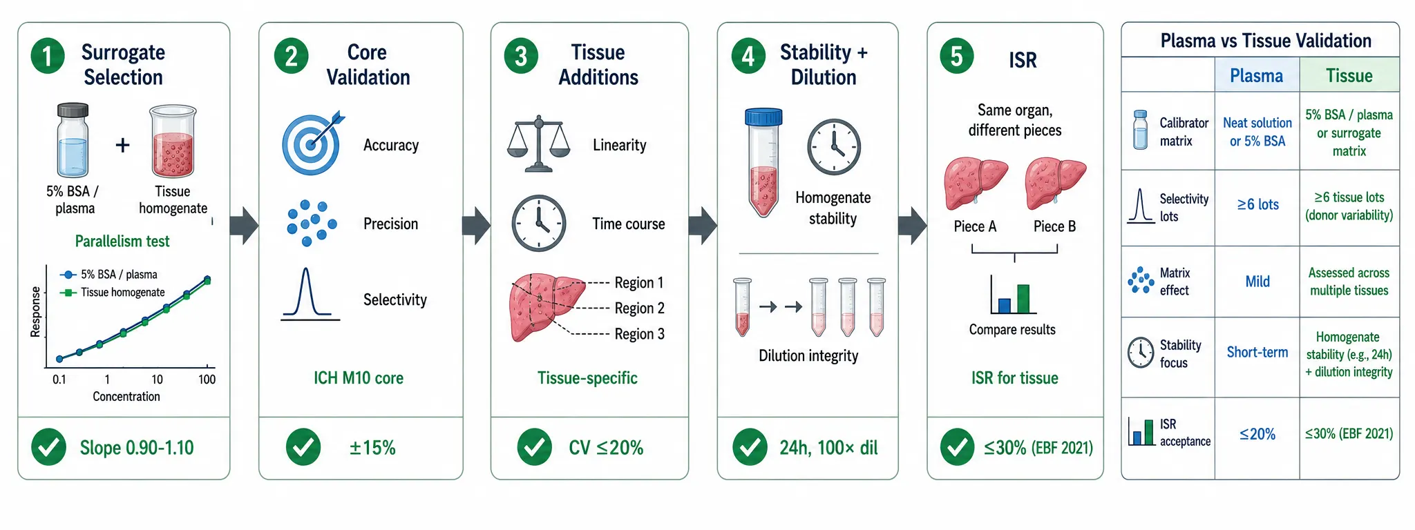Figure 4: Tissue-specific validation workflow. Five panels in sequence: (1) Surrogate matrix selection → parallelism testing; (2) Core validation parameters (accuracy, precision, selectivity, etc.); (3) Tissue-specific additions: weight linearity, time course, regional variability; (4) Homogenate stability + dilution integrity; (5) ISR with sampling location annotation. Green checkmark for each panel, arrows connecting them. Bottom: summary grid showing plasma vs tissue validation differences. Clean white background.

Normalization: ng/g Tissue vs ng/mg Protein — Which, When, Why

After back-calculation, tissue drug concentration can be expressed in two units: ng per gram of tissue (ng/g) or ng per milligram of total protein (ng/mg). The choice affects data comparability and should be made deliberately, not by default.

ng/g tissue is the standard convention for most tissue distribution and toxicokinetic studies. It matches the units of dose (mg/kg) and volume of distribution (L/kg), enabling direct comparison with plasma concentration (ng/mL) for tissue-to-plasma ratio calculation. It requires only accurate tissue weighing — a standard laboratory balance with 0.1 mg readability is adequate for samples ≥50 mg.

ng/mg protein is preferred in three situations: (a) when tissue samples are very small (needle biopsies of 5-20 mg) where weighing error exceeds 20%; (b) when comparing drug concentrations across tissues with very different cellularity, blood content, or hydration (e.g., liver vs adipose); and (c) for intracellular-targeted drugs where the relevant denominator is cellular content, not total tissue mass. Protein normalization corrects for differences in tissue composition that would otherwise confound cross-tissue comparisons.

Typical total protein densities by tissue type: liver 150-200 mg protein per gram tissue, kidney 120-150 mg/g, brain 100-120 mg/g, heart 150-170 mg/g, lung 120-150 mg/g, skeletal muscle 180-200 mg/g, adipose 20-40 mg/g. These are not constants to be assumed — they vary with species, age, and disease state. Measure actual protein concentration on every study using a Bradford or BCA assay on a small homogenate aliquot. Report the measured protein concentration alongside protein-normalized drug concentrations so that downstream consumers (PBPK modelers, clinical pharmacologists) can convert between the two units if needed.

Conversion: ng/mg protein = (ng/g tissue) / (mg protein per g tissue). For a liver sample at 205 ng/g and a measured protein density of 175 mg/g: 205 / 175 = 1.17 ng/mg. The best practice is to report both units when sample characteristics vary or when the intended use of the data (PBPK modeling, cross-species extrapolation) benefits from protein-normalized values. For tissue quantification studies requiring both weight-normalized and protein-normalized concentrations, our internal standard selection and optimization services ensure consistent ionization efficiency across tissue homogenates with varying protein content.

Worked Example: Mouse Liver Quantification from Start to Finish

The following worked example illustrates the complete tissue quantification workflow.

A male CD-1 mouse is dosed with a small-molecule kinase inhibitor at 30 mg/kg PO. At Tmax (2 hours post-dose), the animal is euthanized and the liver is collected, blotted dry, and weighed: 0.52 g. The liver is placed in a 15-mL Precellys tube containing 8.5 g of 1.4-mm ceramic beads and 2.0 mL of ice-cold PBS (pH 7.4), producing a tissue-to-buffer ratio of approximately 1:4 (w/v). The tube is processed in a FastPrep-24 bead beater at 6.0 m/s for 8 minutes at 4°C. After homogenization, the total homogenate volume is measured in a graduated tube: 2.45 mL. The difference (2.45 - 2.00 = 0.45 mL) reflects the tissue volume contribution of approximately 0.87 mL/g — within the expected range for mouse liver.

Sample preparation: 50 μL of homogenate is transferred to a 1.5-mL polypropylene tube. 150 μL of ice-cold acetonitrile containing stable isotope-labeled internal standard (SIL-IS, 50 ng/mL) is added. The tube is vortex-mixed for 1 minute and centrifuged at 14,000 × g for 10 minutes at 4°C. 100 μL of supernatant is transferred to an autosampler vial containing 100 μL of water. 5 μL is injected onto the LC-MS/MS system.

Calibration: eight calibrators (1, 2, 5, 10, 20, 50, 100, 200 ng/mL) are prepared in 5% BSA in PBS (surrogate matrix) by serial dilution from a 1 mg/mL DMSO stock. Four QCs (3, 30, 150, 500 ng/mL) are prepared similarly. Surrogate matrix parallelism was confirmed during method development: slope ratio (tissue homogenate / surrogate) = 0.96, IS-normalized MF 0.94-1.03 across three concentration levels.

LC-MS/MS: Acquity UPLC BEH C18 column (2.1 × 50 mm, 1.7 μm), gradient of 0.1% formic acid in water (A) and 0.1% formic acid in acetonitrile (B) at 0.4 mL/min. Analyte elutes at 1.82 min, SIL-IS at 1.80 min. MRM transition: analyte m/z 488.2 → 345.1 (quantifier), 488.2 → 260.3 (qualifier); IS m/z 492.2 → 349.1. Calibration curve: 1/x² weighted linear regression, r² = 0.9986. Homogenate concentration from the calibration curve: 44.8 ng/mL.

Back-calculation: tissue concentration = homogenate concentration × total homogenate volume / tissue weight = 44.8 ng/mL × 2.45 mL / 0.52 g = 211.2 ng/g. Note: using the buffer volume (2.00 mL) instead of the total volume (2.45 mL) would yield 44.8 × 2.00 / 0.52 = 172.3 ng/g — a 18% underestimate. This is the dilution factor trap described in detail in the tissue homogenization article.

Quality control: all QCs within ±12.1% of nominal. ISR: 6.5% difference (n = 2). Matrix factor: IS-normalized 0.89-1.04. Final reported result: 211 ng/g mouse liver at 2 hours post-dose. When tissue concentrations from multiple organs and time points are combined with plasma concentration data to calculate tissue-to-plasma partition coefficients (Kp) for PBPK modeling, see our article on tissue-to-plasma ratio determination and PBPK integration.

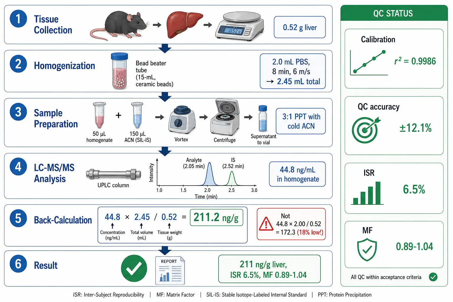Figure 5: Complete tissue quantification workflow diagram. Top-to-bottom visual pipeline: (1) tissue collection → weighing → homogenization (icon of bead beater tube); (2) homogenate → PPT/LLE/SPE → LC-MS/MS injection; (3) calibration curve in surrogate matrix → concentration from instrument (ng/mL); (4) back-calculation equation with numbers: ng/g = ng/mL × total vol / tissue wt; (5) final reported result with QC annotation. Each step has a green checkmark indicating QC passed. Right sidebar: the worked example numbers at each step. Clean white background, green accent (#27AE60).

Frequently Asked Questions

References

Disclaimer: All services and resources mentioned on this site are for research use only (RUO) and are not intended for diagnostic, therapeutic, or clinical applications.

Related Services

• Tissue & Cell Lysate Drug Quantification Services
• LC-MS/MS Single Drug Quantification Services
• Bioanalytical Method Development & Validation Services
• Method Validation — Full, Partial, and Cross-Validation Services
• Custom LC-MS/MS Method Development for Novel Chemical Entities
• Sample Preparation & Processing Method Development
• Bioanalysis of Challenging Compounds & Complex Matrices

References

- Ho S, Gao H. Surrogate matrix: opportunities and challenges for tissue sample analysis. Bioanalysis. 2015;7(18):2419-2433. doi:10.4155/bio.15.161
- Xue YJ, Gao H, Ji QC, et al. Bioanalysis of drug in tissue: current status and challenges. Bioanalysis. 2012;4(21):2637-2653. doi:10.4155/bio.12.252
- Jemal M, Ouyang Z, Xia YQ. Systematic LC-MS/MS bioanalytical method development that incorporates plasma phospholipids risk avoidance, usage of incurred sample and well thought-out chromatography. Biomed Chromatogr. 2010;24(1):2-19. doi:10.1002/bmc.1373
- Van Eeckhaut A, Lanckmans K, Sarre S, Smolders I, Michotte Y. Validation of bioanalytical LC-MS/MS assays: evaluation of matrix effects. J Chromatogr B Analyt Technol Biomed Life Sci. 2009;877(23):2198-2207. doi:10.1016/j.jchromb.2009.01.003
- Matuszewski BK, Constanzer ML, Chavez-Eng CM. Strategies for the assessment of matrix effect in quantitative bioanalytical methods based on HPLC-MS/MS. Anal Chem. 2003;75(13):3019-3030. doi:10.1021/ac020361s
- Fast DM, Kelley M, Viswanathan CT, et al. Workshop report and follow-up — AAPS Workshop on Current Topics in GLP Bioanalysis: Assay Reproducibility for Incurred Samples — implications of Crystal City recommendations. AAPS J. 2009;11(2):238-241. doi:10.1208/s12248-009-9100-9
- International Council for Harmonisation (ICH). ICH guideline M10 on bioanalytical method validation and study sample analysis. 2022. EMA/CHMP/ICH/172948/2019
- Timmerman P, Luedtke S, van Amsterdam P, et al. Incurred sample reproducibility: views and recommendations by the European Bioanalysis Forum. Bioanalysis. 2009;1(6):1049-1056. doi:10.4155/bio.09.108
- Gao H, Ho S, Williams J. LC-MS bioanalysis of drugs in tissue samples. In: Li W, Zhang J, Tse FLS, eds. Handbook of LC-MS Bioanalysis: Best Practices, Experimental Protocols, and Regulations. Hoboken, NJ: John Wiley & Sons; 2013:363-372. doi:10.1002/9781118671276.ch23