Tissue-to-Plasma Ratio (Kp): Determination Methods, Tissue Distribution Study Design, and PBPK Model Integration

A plasma concentration-time curve tells you how much drug circulates in blood. It does not tell you where the drug goes — whether it accumulates in liver, crosses into brain, or partitions into adipose. The tissue-to-plasma partition coefficient, Kp, answers this question: at distribution equilibrium, for every unit of drug in plasma, how many units are in each tissue? Kp is the numeric bridge between the plasma PK that bioanalytical scientists measure and the tissue concentrations that determine efficacy and toxicity. This article covers in vivo Kp determination study design, the blood contamination correction that invalidates Kp <1 if ignored, in vitro and in silico alternatives from equilibrium dialysis to Rodgers-Rowland to machine learning, the lysosomal trapping problem that produces Kp values of 50-500 for basic lipophilic amines, and the integration of Kp into physiologically based pharmacokinetic (PBPK) models that translate preclinical tissue distribution into human dose projections. For the tissue homogenization and LC-MS/MS quantification methods that produce the raw tissue concentration data from which Kp is calculated, see our article on tissue homogenization methods comparison and our article on tissue drug quantification by LC-MS/MS.

What Is Kp and Why It's the Bridge Between Bioanalysis and PBPK

Kp is defined as the ratio of total drug concentration in tissue (Ct) to total drug concentration in plasma (Cp) at distribution equilibrium: Kp = Ct / Cp. A Kp of 10 means the tissue contains ten times more drug per unit mass than plasma. A Kp of 0.3 means the tissue excludes drug relative to plasma — typically due to extensive plasma protein binding with limited tissue binding. Three regimes describe all tissue distribution behavior: Kp >1 indicates tissue accumulation via active uptake transport, lysosomal trapping, or high tissue binding; Kp approximately 1 reflects passive distribution where plasma and tissue binding are balanced; Kp <1 indicates tissue exclusion, most commonly when a drug is highly plasma-protein-bound and tissue binding is low.

The sum of organ-specific Kp values, weighted by organ volumes, determines the volume of distribution at steady state (Vss): Vss = V_plasma + Σ(V_tissue × Kp_tissue). Vss is the single most important PK parameter for predicting human half-life and dosing interval, and it cannot be calculated without Kp. In physiologically based pharmacokinetic (PBPK) models, Kp values populate the tissue compartments and control the arterial-to-tissue concentration gradient that drives tissue drug exposure over time. Without Kp, PBPK is a plasma-only model — useful for clearance, silent on tissue distribution. With Kp, PBPK predicts concentrations in liver (hepatotoxicity risk), heart (QTc risk), brain (CNS efficacy or neurotoxicity), kidney (nephrotoxicity), and any other tissue of toxicological or pharmacological interest.

The Kp concept connects the DMPK article series end-to-end: tissue homogenization methods (A10) and tissue drug quantification by LC-MS/MS (A11) produce the raw tissue concentration data; Kp normalizes those tissue concentrations to plasma, transforming ng/g into dimensionless partition ratios; the ratios feed PBPK models that predict human tissue exposure. For the intracellular analogue of Kp — the cell-to-medium accumulation ratio (Kp,cell) determined from cell lysate LC-MS/MS — see our article on cell lysate drug quantification. Kp is the justification for the entire tissue bioanalysis workflow: if you are measuring tissue drug concentrations, the reason is ultimately to calculate Kp.

In Vivo Kp Determination: Tissue Distribution Study Design

The gold standard for Kp determination is the in vivo tissue distribution study: dose animals, collect blood and tissues at defined time points, homogenize tissues, quantify drug in tissue homogenate and plasma by LC-MS/MS, and calculate Kp. ICH S3A provides the regulatory framework for tissue distribution studies as part of the toxicokinetic assessment, though the study designs described here go beyond the regulatory minimum to produce Kp values suitable for PBPK modeling.

Two fundamentally different approaches exist for calculating Kp from in vivo data: the single-timepoint (terminal) method and the AUC-based method. The terminal method collects blood and tissues at a single time point in the terminal elimination phase, when plasma and tissue concentrations are assumed to decline in parallel — i.e., they share the same terminal elimination rate constant (λz). Under this pseudo-equilibrium condition, the concentration ratio at any terminal time point equals the steady-state ratio: Kp_terminal = Ct(t) / Cp(t) for t in the terminal phase. The terminal method requires only one time point per animal, making it efficient for screening, and is widely used in early discovery. Its limitation is the pseudo-equilibrium assumption: if drug efflux from tissue is slower than plasma elimination — as occurs for lysosomotropic drugs, drugs with high tissue binding, or drugs in poorly perfused tissues — the tissue concentration lags behind plasma, and the terminal ratio overestimates the true steady-state Kp. The magnitude of overestimation equals the tissue-to-plasma half-life ratio; for adipose tissue, this can be 5-fold or more.

The AUC-based method calculates Kp as the ratio of the area under the tissue concentration-time curve to the area under the plasma concentration-time curve over the same time interval: Kp_AUC = AUC_tissue / AUC_plasma. This method requires no equilibrium assumption and is always mathematically correct — it represents the time-averaged partition coefficient. The cost is experimental: full concentration-time profiles must be collected in every tissue, requiring 5-8 time points covering absorption, distribution, and elimination phases, with 3 animals per time point per tissue. For a study with 8 time points, 10 tissues, and 3 animals per time point, the tissue collection and bioanalytical burden is substantial. In practice, the terminal method is used for screening and rank-ordering across compounds, while the AUC method is reserved for lead candidates where accurate human PK prediction depends on accurate Kp.

Time-point selection for the terminal method: a minimum of 3 time points (Tmax, 2× Tmax, 4× Tmax) should be collected to confirm that tissue and plasma λz are parallel. If the tissue λz differs from the plasma λz by more than 20%, terminal Kp is unreliable and the AUC method should be used. For cassette (N-in-1) dosing, 5-10 compounds are co-administered at low individual doses (total combined dose typically ≤5 mg/kg) and measured simultaneously in each tissue by multiplexed LC-MS/MS. Cassette dosing dramatically reduces animal use — 9 animals for 10 compounds versus 90 — but requires three controls: (a) include a positive-control P-gp substrate such as digoxin to verify that cassette competition at intestinal and hepatic transporters is not occurring; (b) keep total cassette dose low enough that combined exposures stay within linear PK range; (c) the LC-MS/MS method must chromatographically resolve all cassette compounds and their isomers or isobars. Cassette Kp values that agree with discrete-dose Kp values (within 2-fold) are considered valid for screening; compounds showing >2-fold deviation require discrete-dose confirmation.

Tissues to collect for a comprehensive Kp determination, consistent with ICH S3A guidance: liver, kidney, brain, heart, lung, spleen, skeletal muscle, adipose (white and brown separately in rodents), gonads (testes or ovaries), and bone marrow. Add target organs relevant to the pharmacology or toxicology of the compound — thyroid for a tyrosine kinase inhibitor with thyroid toxicity signal, pancreas for a GLP-1 receptor agonist, skin for a compound with dermal toxicity findings. For tissue distribution studies supporting PBPK model development, our tissue and cell lysate drug quantification services provide comprehensive multi-tissue LC-MS/MS analysis with both terminal and AUC-based Kp calculation. For the bioanalytical method validation that qualifies the tissue LC-MS/MS assay generating the concentration data from which Kp is derived, our method validation services include full ICH M10 validation for tissue homogenate matrices.

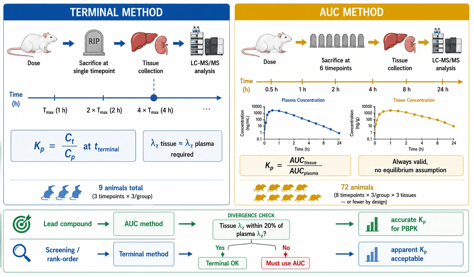Figure 1: Tissue distribution study design comparison. Two panels: Terminal method — single timepoint in elimination phase, tissue and plasma decline in parallel, equation Kp = Ct/Cp at t_terminal. AUC method — 5-8 timepoints, full profiles, equation Kp = AUC_tissue/AUC_plasma. Bottom: animal number comparison table (terminal 9 vs AUC 72 per compound). Right sidebar: parallel λz check — tissue λz within 20% of plasma λz → terminal OK; >20% → must use AUC. Decision tree: lead compound → AUC; screening/rank-order → terminal. Clean white background, blue accent (#2980B9).

The Blood Contamination Correction

When tissue is collected from an animal, it contains residual blood — drug in that blood is measured by LC-MS/MS and attributed to tissue, but it is not tissue drug. Residual blood volume in unperfused tissues ranges from approximately 0.5% (muscle, adipose) to 20% (lung). Representative values: liver 10-15% of tissue weight is residual blood, kidney 8-12%, lung 15-20%, heart 6-10%, brain 1-2% (blood-brain barrier limits blood volume), muscle 0.5-2%, adipose 0.5-1%. Perfusion with saline via the portal vein (liver), renal artery (kidney), or cardiac puncture (whole-body) removes most residual blood and should be documented in the study report. Perfused tissues are the standard for regulatory tissue distribution studies.

The correction formula is: Kp_corrected = (Kp_apparent − V_blood × Rb) / (1 − V_blood), where V_blood is the fraction of tissue weight that is residual blood and Rb is the blood-to-plasma concentration ratio. Equivalently, on a concentration basis: C_tissue_corrected = (C_tissue_measured − C_blood × V_blood) / (1 − V_blood). The magnitude of the correction depends on the Kp regime. When Kp is large (Kp ≥ 10), residual blood contributes negligibly to the tissue measurement — a 10% blood volume even at plasma-equivalent concentration adds at most 10% to the apparent Kp, producing a minor correction. When Kp is approximately 1, the correction is noticeable but moderate. When Kp is less than 1 — meaning tissue concentration is lower than plasma concentration — residual blood can dominate the measurement. Example: Kp_apparent = 0.3, V_blood = 0.10 (10% residual blood in liver), Rb = 2 (drug concentrates 2-fold in blood cells relative to plasma). Kp_corrected = (0.3 − 0.10 × 2) / (1 − 0.10) = (0.3 − 0.20) / 0.90 = 0.111. The apparent Kp overestimates the true tissue Kp by 170% — reporting Kp = 0.3 when the true value is 0.11. Every Kp less than 1 must be blood-corrected. Skipping this correction for Kp <1 can reverse the conclusion: a drug that appears to achieve tissue concentrations 30% of plasma (suggesting some tissue penetration) actually achieves only 11% (suggesting near-exclusion). For tissue Kp calculations requiring blood contamination correction across multiple tissues, our single drug quantification services include blood-corrected Kp values with Rb and V_blood documented for each tissue.

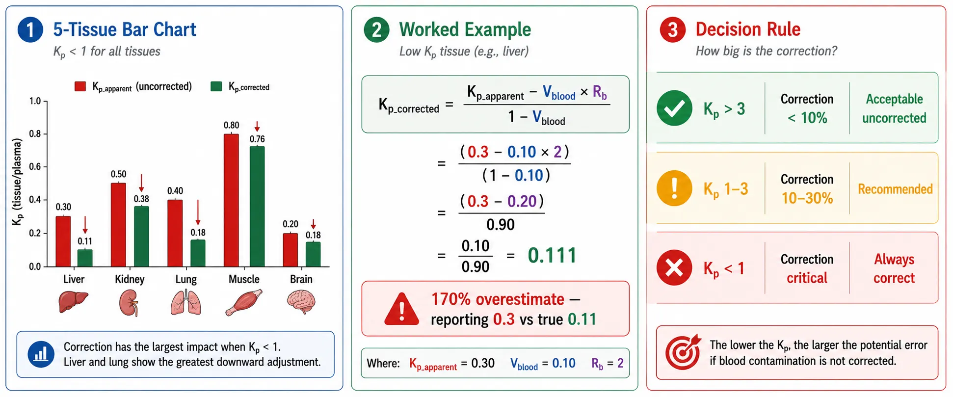Figure 2: Blood contamination correction — before/after comparison. Left: bar chart showing Kp_apparent vs Kp_corrected across 5 tissues with Kp <1, showing dramatic downward corrections. Center: worked example calculation (Kp_apparent=0.3, V_blood=0.10, Rb=2 → Kp_corrected=0.11, 170% overestimate). Right: decision rule — "Kp <1? Always correct. Kp >>10? Acceptable uncorrected." Color-coded: green (Kp >3, minor correction), amber (Kp 1-3, moderate), red (Kp <1, critical). Clean white background.

In Vitro and In Silico Kp Prediction Methods

In vivo tissue distribution studies remain the reference method for Kp, but they are animal-intensive, costly, and cannot provide human tissue Kp values directly. Three categories of alternatives exist, each trading accuracy for throughput.

In vitro — Tissue homogenate equilibrium dialysis. Blank tissue is homogenized in phosphate buffer, spiked with drug, and dialyzed against buffer to measure the unbound fraction in tissue homogenate (fu_tissue). Kp is then estimated from the ratio of unbound fraction in plasma to unbound fraction in tissue: Kp = fup / fu_tissue. The method is rapid, uses small amounts of blank tissue, and can be performed in 96-well format for high-throughput screening. Its limitation is fundamental: homogenization destroys cellular architecture, eliminating pH gradients (lysosomes, mitochondria), membrane potentials, and transporter activity. For passively distributed drugs without significant transporter involvement, the fu_tissue method predicts Kp within 2-fold of in vivo values. For drugs that are substrates of uptake transporters — OATP1B1, OATP1B3, OCT1, OAT1/3 — the homogenate method predicts Kp values that are 10- to 50-fold lower than in vivo, because active intracellular accumulation is absent in the homogenate. The method systematically underpredicts Kp for transporter substrates and overpredicts it for efflux transporter substrates that would be actively excluded in vivo.

In vitro — Precision-cut tissue slices. Tissue cores (8 mm diameter) are sliced to 200-300 µm thickness on a microtome, incubated in oxygenated buffer at 37°C with drug, and the slice-to-medium concentration ratio measured over time. Tissue slices preserve three-dimensional architecture, cell-cell junctions, heterogeneous cell populations, and functional transporter activity for 4-6 hours post-preparation. The slice-to-medium ratio at steady state approximates Kp. Limitations: oxygen and drug diffusion through the slice thickness limits applicability to tissues with high metabolic rate (liver slices consume oxygen faster than it diffuses, creating a hypoxic core); slice viability declines measurably after 4-6 hours; inter-slice variability is substantial (CV 20-40%). Tissue slices are most useful for liver Kp determination where transporter activity must be preserved and where the comparison between slice and homogenate Kp directly quantifies the transporter contribution.

In silico — Rodgers-Rowland equations (2005-2006). The Rodgers-Rowland method predicts Kp from a compound's physicochemical properties — logP, pKa, plasma protein binding (fup) — and the known phospholipid and neutral lipid composition of each tissue. It models tissue distribution as partitioning into five compartments: neutral phospholipids, neutral lipids, tissue water, plasma protein-associated drug, and (for basic drugs) acidic phospholipid binding. The equations are implemented by default in Simcyp and are the most widely used in silico Kp prediction method in pharmaceutical R&D. R-R predicts Kp well (within 2-3 fold) for neutral and acidic drugs. It systematically underpredicts Kp for moderate-to-strong bases because it does not account for lysosomal trapping — the accumulation of protonated basic drug in acidic intracellular compartments. R^2 between predicted and observed Kp is typically 0.3-0.5 across structurally diverse compound sets. For PBPK model development integrating multiple Kp prediction methods, our bioanalytical method development and validation services support the in vitro and in vivo studies that generate the input data for in silico Kp prediction. For tissue homogenate dialysis and tissue slice uptake experiments in support of Kp determination, our sample preparation and processing services include validated protocols for tissue homogenization, equilibrium dialysis, and tissue slice preparation.

In silico — Machine learning methods. Graph neural network and random forest approaches have been applied to Kp prediction using literature datasets of tissue-to-plasma ratios across multiple compounds and tissues. A 2024 study by Handa et al. (JCIM) used a two-stage repeated random forest method to predict Kp for 119 compounds across 9 tissues, outperforming both conventional regression and message-passing neural networks for most tissues. Reported R^2 values for ML-based tissue Kp prediction typically reach 0.7-0.8, substantially exceeding the Rodgers-Rowland equations (R^2 0.3-0.5). However, the training data come from heterogeneous literature sources with different study designs, species, time points, and correction methods — the models may be learning laboratory noise as much as drug-tissue interactions. As of 2025-2026, ML Kp prediction is a promising screening tool but is not accepted by regulatory agencies for PBPK submissions. The appropriate use case is early discovery ranking: across hundreds of compounds, ML-Kp identifies those most likely to show extreme tissue accumulation or exclusion, triggering confirmatory in vivo or in vitro studies.

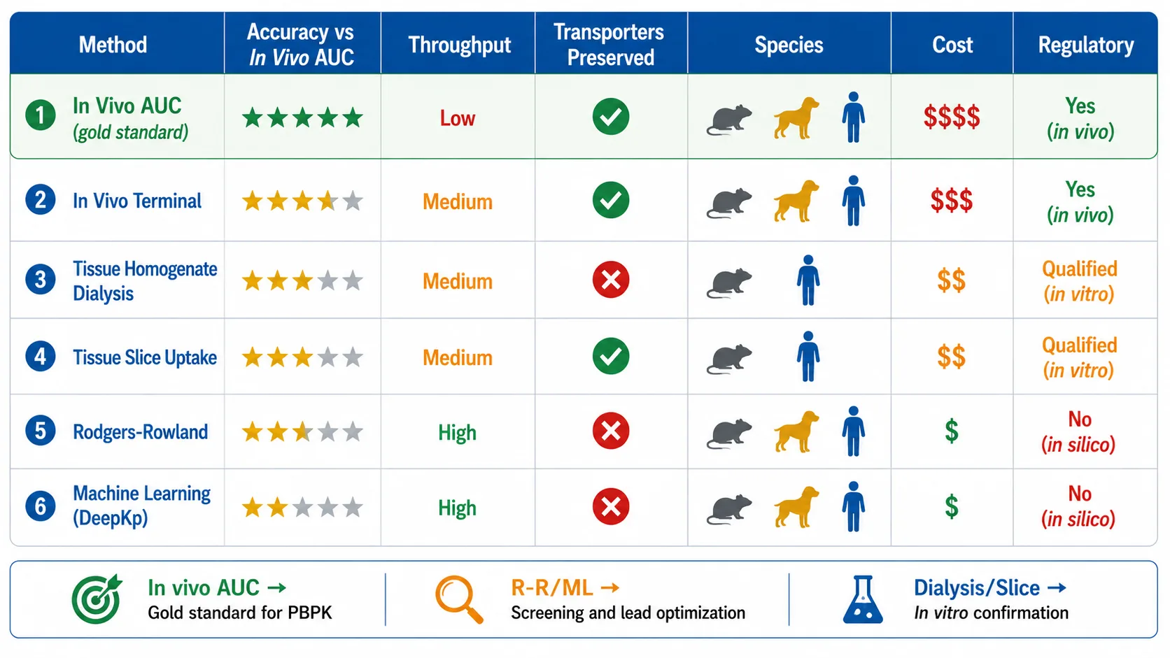Figure 3: Kp method comparison matrix. 5-row grid: In vivo (AUC), in vivo (terminal), tissue homogenate dialysis, tissue slice uptake, Rodgers-Rowland, machine learning. Columns: accuracy vs in vivo AUC (stars 1-5), throughput (low/med/high), transporter preserved (yes/no), species applicability (rat/dog/human), cost ($-$$$$). Rodgers-Rowland and ML rows color-coded as in silico. Green highlight on in vivo AUC as gold standard. Clean white background.

The Lysosomal Trapping Problem

Lysosomes maintain an internal pH of 4.5-5.0 via vacuolar ATPase (V-ATPase) proton pumping, approximately 100- to 1,000-fold more acidic than the cytoplasmic pH of 7.2. Basic drugs with pKa values in the range 7-9 cross lysosomal membranes by passive diffusion in their neutral (unprotonated) form. Once inside the acidic lysosomal lumen, they become protonated, acquire a positive charge, and cannot cross back across the lipid bilayer — the charged form is membrane-impermeable. This ion-trapping mechanism, combined with the pH gradient, produces lysosomal accumulation ratios of 100- to 1,000-fold relative to cytoplasm for drugs with the right physicochemical profile: pKa 7-9 (basic amine), logP >3 (sufficient membrane permeability), and a protonatable nitrogen atom.

The Kp consequences are dramatic. Liver Kp values for lysosomotropic drugs exceed any in silico prediction: amiodarone (antiarrhythmic, pKa ∼8.7, logP ∼7.0) has a measured liver Kp of approximately 50-500; chloroquine (antimalarial, pKa ∼8.4/10.8, logP ∼4.6) concentrates in liver and spleen at Kp values of 100-500; fluoxetine (SSRI, pKa ∼9.8, logP ∼4.1) and propranolol (beta-blocker, pKa ∼9.4, logP ∼3.5) show liver Kp values 10- to 50-fold above R-R predictions. The Rodgers-Rowland equations predict none of this because they lack a lysosomal compartment.

Detection is straightforward: treat cells or tissue slices with bafilomycin A1 (a specific V-ATPase inhibitor that collapses the lysosomal pH gradient) at 100 nM for 30-60 minutes before and during drug incubation. If tissue uptake decreases significantly (typically >50%) in the presence of bafilomycin A1, lysosomal trapping is confirmed. Ammonium chloride (10-20 mM) is a cheaper but less specific alternative that neutralizes acidic compartments. The experimental comparison is: measure in vivo Kp, measure fu_tissue Kp by homogenate dialysis, and compare. If the in vivo Kp / fu_tissue Kp ratio exceeds 3, active intracellular accumulation — usually transporter-mediated uptake or lysosomal trapping — is present. Bafilomycin A1 treatment distinguishes between the two: if bafilomycin eliminates the discrepancy, it is lysosomal trapping; if it does not, transporter-mediated uptake (OATP, OCT, OAT) is the likely mechanism.

A practical rule: any compound with a basic amine (pKa >7), logP >3, and a predicted liver Kp by Rodgers-Rowland of less than 10 should be suspected of lysosomal trapping. Either measure in vivo Kp or apply an empirical correction factor of 3-10× to the R-R prediction based on structural analogues with known lysosomal trapping behavior.

For liver Kp studies requiring transporter substrate assessment and lysosomal trapping evaluation, our complex biological matrices analysis services include bafilomycin A1 control experiments to distinguish transporter-mediated from pH-driven intracellular accumulation.

Species Differences in Kp and Allometric Scaling

Kp is species-dependent because tissue composition differs across species. The most consequential difference is adipose tissue: rodents have substantial brown and beige adipose depots with higher mitochondrial density, higher phospholipid-to-neutral-lipid ratio, and greater blood perfusion than human white adipose tissue. Lipophilic drugs (logP >4) that partition primarily into neutral lipids show systematically lower adipose Kp in humans than rodents — the human white adipose tissue has a higher neutral lipid fraction per gram, diluting drug concentration and producing a lower Kp per unit tissue weight. Conversely, brain Kp differences arise from differences in white-to-gray matter ratio (rodent brain is approximately 25% white matter, human approximately 50%) and species differences in blood-brain barrier transporter expression.

Muscle, the tissue that dominates Vss by mass (approximately 40% of body weight in both rats and humans), has relatively conserved phospholipid composition across species. Muscle Kp tends to be the most cross-species consistent Kp value. Liver and kidney Kp differences are driven primarily by species differences in transporter expression — rodent hepatocytes express higher levels of OATP1A/1B transporters per gram of liver than human hepatocytes, leading to systematically higher rodent liver Kp for OATP substrates.

The allometric scaling trap: Vss is commonly scaled allometrically across species (Vss ∝ BW^b) without considering that Vss = Σ(V_tissue × Kp_tissue). If individual Kp values differ across species, the allometric exponent is a composite of species-dependent tissue Kp values — it reflects body weight only coincidentally. When Kp is species-invariant, Vss scales with organ weights (which scale allometrically with body weight), and allometry works. When Kp differs — as for lipophilic drugs (adipose Kp species effect) or OATP substrates (liver Kp species effect) — allometric Vss scaling from rodent to human can fail by 3- to 5-fold.

The recommended strategy: measure rat Kp in vivo using the terminal or AUC method across the standard tissue panel. Predict human Kp using the Rodgers-Rowland or Kp/mem equations with human fup, human pKa, and human tissue composition parameters. Validate the in silico prediction method against the measured rat data — if rat predicted Kp agrees with rat measured Kp within 2-fold across most tissues, the method is calibrated for human prediction. If human predicted Kp differs from rat measured Kp by more than 3-fold for any tissue, flag that tissue for PBPK sensitivity analysis. For muscle (the dominant Vss contributor), a Kp difference of >2-fold between species warrants a dedicated human tissue in vitro study (hepatocyte uptake for liver, tissue homogenate binding for muscle).

For cross-species tissue distribution studies supporting human PK prediction, our tissue and cell lysate drug quantification services provide multi-species tissue Kp determination with cross-species comparison and human PBPK-ready Kp values.

From Kp to PBPK: The Integration Workflow

In a PBPK model, the mass balance equation for each tissue compartment is: dCt/dt = Qt × (Ca − Ct/Kp) − CLint,t × fut × Ct, where Qt is tissue blood flow, Ca is arterial blood concentration, Ct is tissue concentration, Kp is the tissue-to-plasma partition coefficient, CLint,t is intrinsic tissue clearance, and fut is the unbound fraction in tissue. The term Ct/Kp converts tissue concentration back to the equivalent plasma (venous outflow) concentration that drives the arterial-to-tissue gradient. Kp controls both the rate of tissue equilibration (higher Kp → larger tissue sink → slower equilibration) and the steady-state tissue-to-plasma ratio.

The Vss expansion connects individual Kp values to the whole-body PK parameter: Vss = V_plasma + V_liver·Kp_liver + V_kidney·Kp_kidney + V_brain·Kp_brain + V_heart·Kp_heart + V_lung·Kp_lung + V_muscle·Kp_muscle + V_adipose·Kp_adipose + V_spleen·Kp_spleen + V_skin·Kp_skin + V_bone·Kp_bone + ... Muscles (40% body weight) and adipose (variable, 10-40% of body weight depending on species and strain) contribute the largest terms to Vss for most drugs. Liver and kidney have small masses (approximately 3-5% and 0.5-1% of body weight, respectively) but receive the highest perfusion — they dominate the distribution kinetics (rate of equilibration) but contribute modestly to Vss magnitude.

The nine-step Kp-to-PBPK integration pipeline: (1) Measure tissue concentrations by LC-MS/MS in the tissue distribution study, using validated homogenization (see tissue homogenization methods) and quantification methods (see tissue drug quantification by LC-MS/MS). (2) Measure plasma concentrations at the same time points. (3) Calculate Kp for each tissue using the AUC method (preferred) or terminal method (confirm parallel λz). (4) Apply blood contamination correction, particularly for tissues with Kp <1. (5) Enter Kp values into PBPK software (Simcyp, GastroPlus, PK-Sim) populating the tissue compartments. (6) Run the plasma concentration-time simulation using the compound's clearance, volume, and absorption parameters. (7) Compare simulated versus observed plasma PK — if the plasma profile is well-described, the model's distribution component (Kp) is internally consistent with the observed plasma PK. (8) If plasma fit is poor, perform sensitivity analysis: which tissue Kp has the greatest impact on Vss and plasma half-life? Typically muscle (Vss) and liver (first-pass extraction). Adjust the highest-sensitivity Kp within the plausible range and re-simulate. (9) Once plasma PK is validated, the tissue concentration-time profiles predicted by the model are credible — report the predicted human tissue exposure at the anticipated therapeutic dose alongside the corresponding plasma exposure.

Common Kp adjustments: if simulated Vss is lower than observed, increase muscle Kp (largest Vss contributor). If simulated half-life is shorter than observed, increase adipose Kp (slowest-equilibrating tissue, prolongs terminal half-life). If simulated oral bioavailability deviates from observed, check liver Kp — liver Kp affects first-pass extraction by controlling the drug concentration presented to hepatic metabolizing enzymes. For complete PBPK model building from tissue distribution data, our bioanalytical method development and validation services support the generation of regulatory-quality tissue concentration data that feeds directly into PBPK modeling platforms. For the stable isotope-labeled internal standards that correct for tissue-specific matrix effects in multi-tissue Kp studies, our internal standard selection and optimization services ensure accurate quantification across diverse tissue matrices.

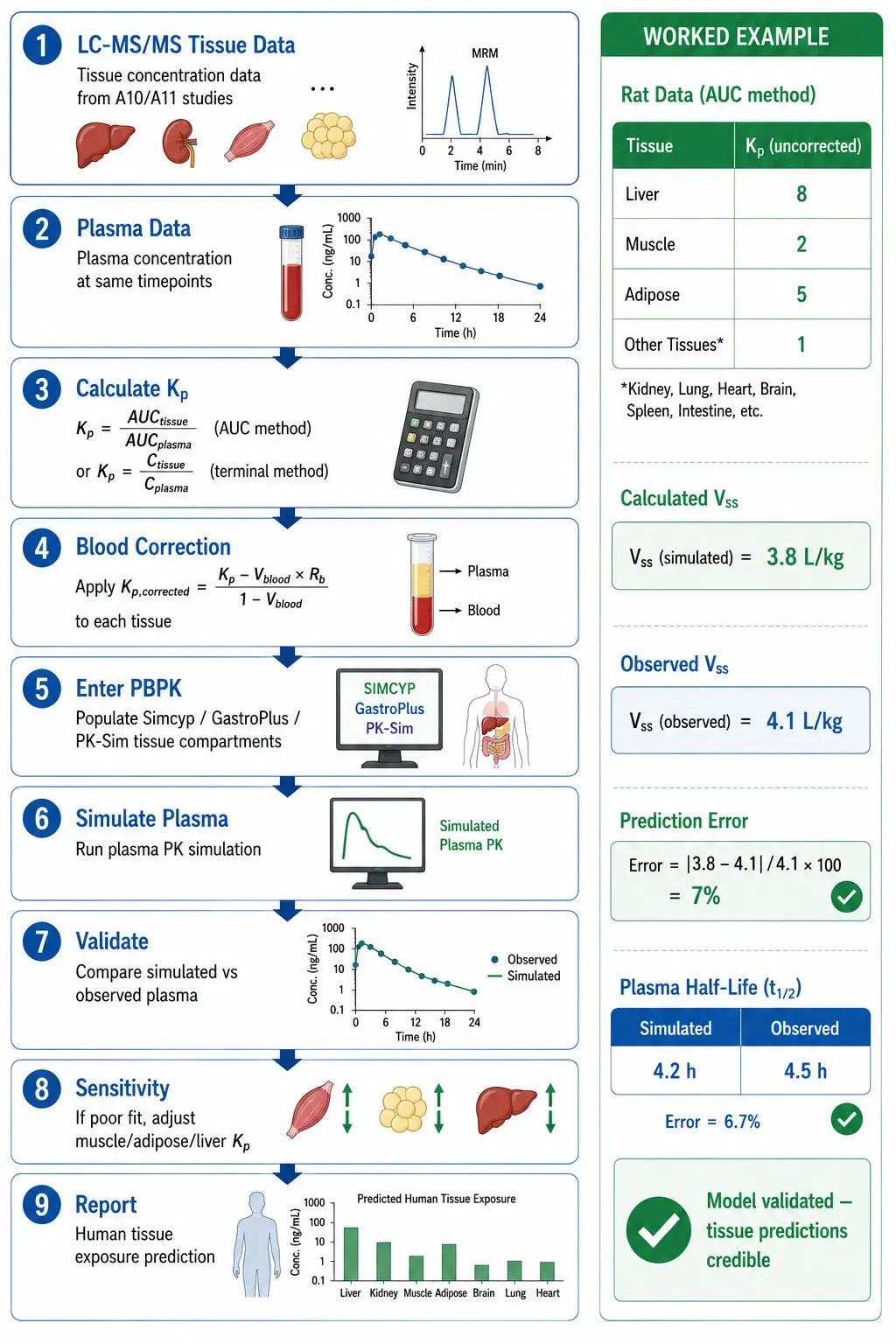Figure 4: Kp-to-PBPK 9-step pipeline. Top-to-bottom workflow: LC-MS/MS tissue data → plasma data → Kp calculation → blood correction → enter PBPK → simulate plasma → validate vs observed → sensitivity analysis → report tissue predictions. Right sidebar: worked example with real numbers showing rat liver Kp = 8, muscle Kp = 2, calculated Vss = 3.8 L/kg vs observed 4.1 L/kg (7% error). Decision nodes: plasma fit good → tissue predictions credible; plasma fit poor → adjust muscle or liver Kp → re-simulate. Clean white background, green accent (#27AE60).

Practical Pitfalls in Kp Determination

Non-steady-state sampling. Kp is defined at distribution equilibrium. Sampling before equilibrium — at Tmax or on the absorption phase — underestimates Kp for tissues that equilibrate slowly because drug is still entering the tissue. Sampling during early elimination when tissue concentrations lag behind plasma overestimates Kp because the tissue has not yet cleared drug in parallel. Validate pseudo-equilibrium by comparing tissue and plasma λz: if they differ by more than 20%, equilibrium has not been reached and terminal Kp is unreliable. The AUC method avoids this issue entirely but requires more sampling.

Tissue heterogeneity. Drug concentration can differ substantially across regions of the same organ: portal versus central regions of the liver lobule, cortex versus medulla of the kidney, gray versus white matter of the brain. Standardize the sampling location within each organ and document it in the study report. For liver, sample from the largest lobe (left lateral lobe in rodents) consistently. For kidney, separate cortex and medulla if transporter-mediated regional differences are expected (e.g., OCT2 substrates concentrate in proximal tubules). For brain, homogenize whole brain or report regional Kp separately.

Temperature-dependent plasma protein binding. Plasma is typically processed at 4°C for stability, but fup is measured at 37°C. If fup is temperature-sensitive — as for some lipophilic drugs where binding to alpha-1-acid glycoprotein (AAG) changes with temperature — the plasma free fraction at 4°C during sample processing differs from the in vivo free fraction at 37°C. This does not directly affect total Kp (which uses total concentrations), but it affects the free tissue concentration calculation (Ct,free = Ct × fut) and the comparison to in vitro pharmacology data measured at 37°C.

Perfusion status. If tissues are not perfused, the measured "tissue" drug concentration includes drug in residual blood. When C_blood substantially exceeds C_tissue — as for highly plasma-protein-bound drugs — residual blood can dominate the tissue measurement and invalidate Kp. If perfusion is logistically impossible (e.g., discovery screening), apply the blood contamination correction for every tissue and flag unperfused Kp values as apparent. A Kp reported without perfusion status is ambiguous.

Metabolite interference. LC-MS/MS methods quantify the parent drug, but if the tissue contains metabolite that undergoes back-conversion to parent during sample processing (e.g., N-oxide reduction, glucuronide hydrolysis), the measured parent concentration is inflated and Kp is overestimated. Check tissue stability: spike parent and major metabolite standards into blank tissue homogenate, process using the study method, and confirm no interconversion. For unstable metabolites (acyl glucuronides, N-oxides), add enzyme inhibitors (e.g., saccharic acid lactone for glucuronidases) to the homogenization buffer. For quantitative tissue analysis with metabolite stability assessment, our custom LC-MS/MS method development services include tissue-specific metabolite interference testing as part of method validation.

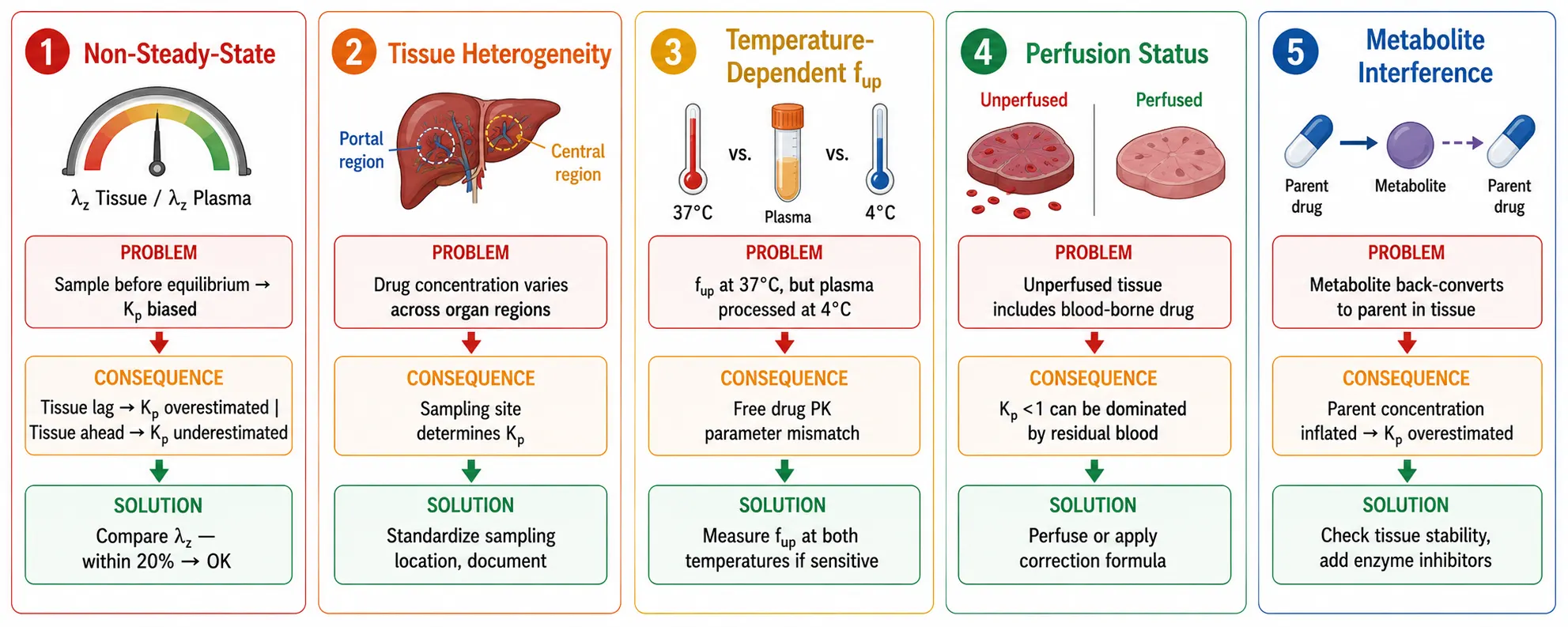Figure 5: Practical pitfalls summary infographic. Five-panel layout: (1) Non-steady-state — tissue/plasma λz comparison; (2) Heterogeneity — regional sampling standardized; (3) Temperature fup — 37°C vs 4°C; (4) Perfusion — blood contamination warning; (5) Metabolite interference — parent-metabolite interconversion. Each panel shows the problem → consequence → solution in 3 lines. Clean white background, red-amber-green severity indicators.

Frequently Asked Questions

References

Disclaimer: All services and resources mentioned on this site are for research use only (RUO) and are not intended for diagnostic, therapeutic, or clinical applications.

Related Services

• Tissue & Cell Lysate Drug Quantification Services
• LC-MS/MS Single Drug Quantification Services
• Bioanalytical Method Development & Validation Services
• Method Validation — Full, Partial, and Cross-Validation Services
• Custom LC-MS/MS Method Development for Novel Chemical Entities
• Sample Preparation & Processing Method Development
• Bioanalysis of Challenging Compounds & Complex Matrices

References

- Rodgers T, Leahy D, Rowland M. Physiologically based pharmacokinetic modeling 1: predicting the tissue distribution of moderate-to-strong bases. J Pharm Sci. 2005;94(6):1259-1276. doi:10.1002/jps.20322
- Rodgers T, Rowland M. Physiologically based pharmacokinetic modelling 2: predicting the tissue distribution of acids, very weak bases, neutrals and zwitterions. J Pharm Sci. 2006;95(6):1238-1257. doi:10.1002/jps.20502
- Poulin P, Theil FP. Prediction of pharmacokinetics prior to in vivo studies. 1. Mechanism-based prediction of volume of distribution. J Pharm Sci. 2002;91(1):129-156. doi:10.1002/jps.10005
- Berezhkovskiy LM. Volume of distribution at steady state for a linear pharmacokinetic system with peripheral elimination. J Pharm Sci. 2004;93(6):1628-1640. doi:10.1002/jps.20073
- Jones HM, Gardner IB, Watson KJ. Modelling and PBPK simulation in drug discovery. AAPS J. 2009;11(1):155-166. doi:10.1208/s12248-009-9088-1
- Hallifax D, Foster JA, Houston JB. Prediction of human metabolic clearance from in vitro systems: retrospective analysis and prospective view. Pharm Res. 2010;27(10):2150-2161. doi:10.1007/s11095-010-0218-3
- Guo Y, Chu X, Parrott NJ, Brouwer KLR, Hsu V, Nagar S, et al. Advancing Predictions of Tissue and Intracellular Drug Concentrations Using In Vitro, Imaging and Physiologically Based Pharmacokinetic Modeling Approaches. Clin Pharmacol Ther. 2018;104(5):865-889. doi:10.1002/cpt.1183
- De Buck SS, Sinha VK, Fenu LA, Nijsen MJ, Mackie CE, Gilissen RAHJ. Prediction of human pharmacokinetics using physiologically based modeling: a retrospective analysis of 26 clinically tested drugs. Drug Metab Dispos. 2007;35(10):1766-1780. doi:10.1124/dmd.107.015644
- Chu X, Bleasby K, Evers R. Species differences in drug transporters and implications for translating preclinical findings to humans. Expert Opin Drug Metab Toxicol. 2013;9(3):237-252. doi:10.1517/17425255.2013.741589
- Handa K, Yoshimura S, Kageyama M, Iijima T. Development of Novel Methods for QSAR Modeling by Machine Learning Repeatedly: A Case Study on Drug Distribution to Each Tissue. J Chem Inf Model. 2024;64(9):3662-3669. doi:10.1021/acs.jcim.4c00046